Jupyter Notebook Tutorial
Roughly, the design idea of mdciao is that:
The CLI offers pre-packaged analysis pipelines that are essentially one-shot tools. They are an entry-point for non-experts and do not require any Python scripting knowledge. CLI tools are still highly customizable (check
mdc_*.py -hormdc_examples.py), but offer only some of themdciao-functionalities.The Python API, on the other hand, exposes:
CLI-equivalent functions via the
mdciao.clisubmodule. Here you’ll find evertying that the CLI offers, only as regular Python functions. This provides scripting flexibility, with the added value that now input and outputs are normal Python objects that can be further manipulated, bymdciaoor any other Python module of your liking.Other standalone submodules that the CLI uses under the hood, and that the user can access directly for any other scripting purpuse: plotting methods, alignment/sequence methods, nomenclature methods, PDB-methods etc.
Note
The API has reached stable status. Future changes/breaks should be easy to handle if you are using mdciao in API mode.
For clarity, this notebook loosely follows the same structure as the Overview section of the mdciaodocumentation. Other notebooks deal with concepts beyond this and/or advanced pipelines.
If you want to run this notebook on your own, please download and extract the data from here first. You can download it:
using the browser
using the terminal with
wget http://proteinformatics.org/mdciao/mdciao_example.zip; unzip mdciao_example.zipusing mdciao’s own method mdciao.examples.fetch_example_data
If you want to take a 3D-look at this data, you can do it here.
[1]:
import mdciao, os
if not os.path.exists("mdciao_example"):
    mdciao.examples.fetch_example_data()
Unzipping to 'mdciao_example'
Basic Usage
Now we replicate the CLI command:
mdc_neighborhoods.py top.pdb traj.xtc --residues L394 -nf #nf: don't use fragments
but in API mode. We use the method cli.residue_neighborhoods:
[2]:
neighborhoods = mdciao.cli.residue_neighborhoods("L394",
                                                 "mdciao_example/traj.xtc",
                                                 topology="mdciao_example/top.pdb",
                                                 fragments=None)
Will compute contact frequencies for (1 items):
mdciao_example/traj.xtc
 with a stride of 1 frames
Using method 'None' these fragments were found
fragment 0 with   1044 AAs     LEU4 (   0) -   P0G395 (1043) (0) resSeq jumps

Will compute neighborhoods for the residues
L394
excluding 4 nearest neighbors

   residue      residx    fragment      resSeq
    LEU394         353           0         394

Performing a first pass on 1039 residue pairs to compute lower bounds on residue-residue distances via residue-COM distances:
Reduced to only 43 residue pairs for the computation of actual residue-residue distances:
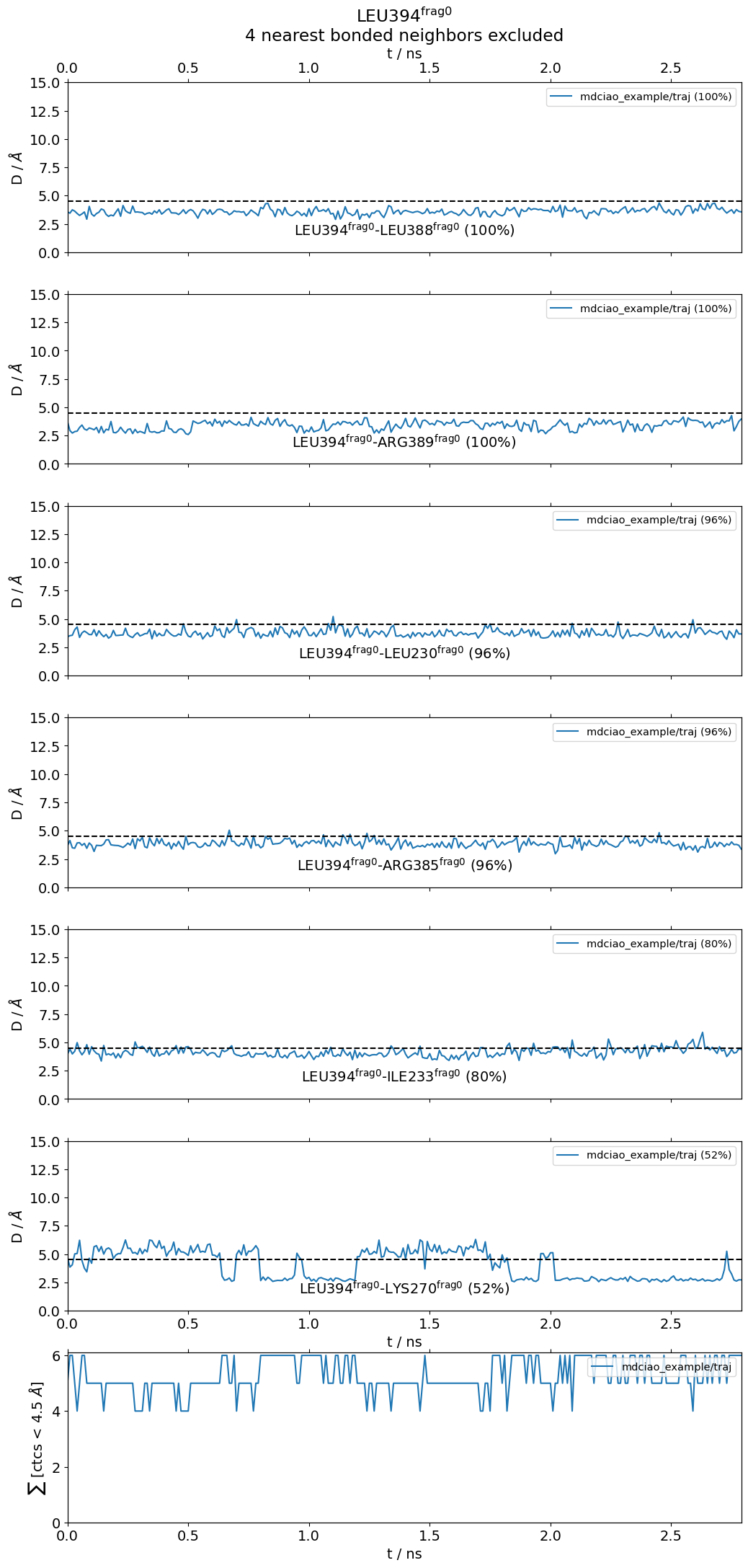
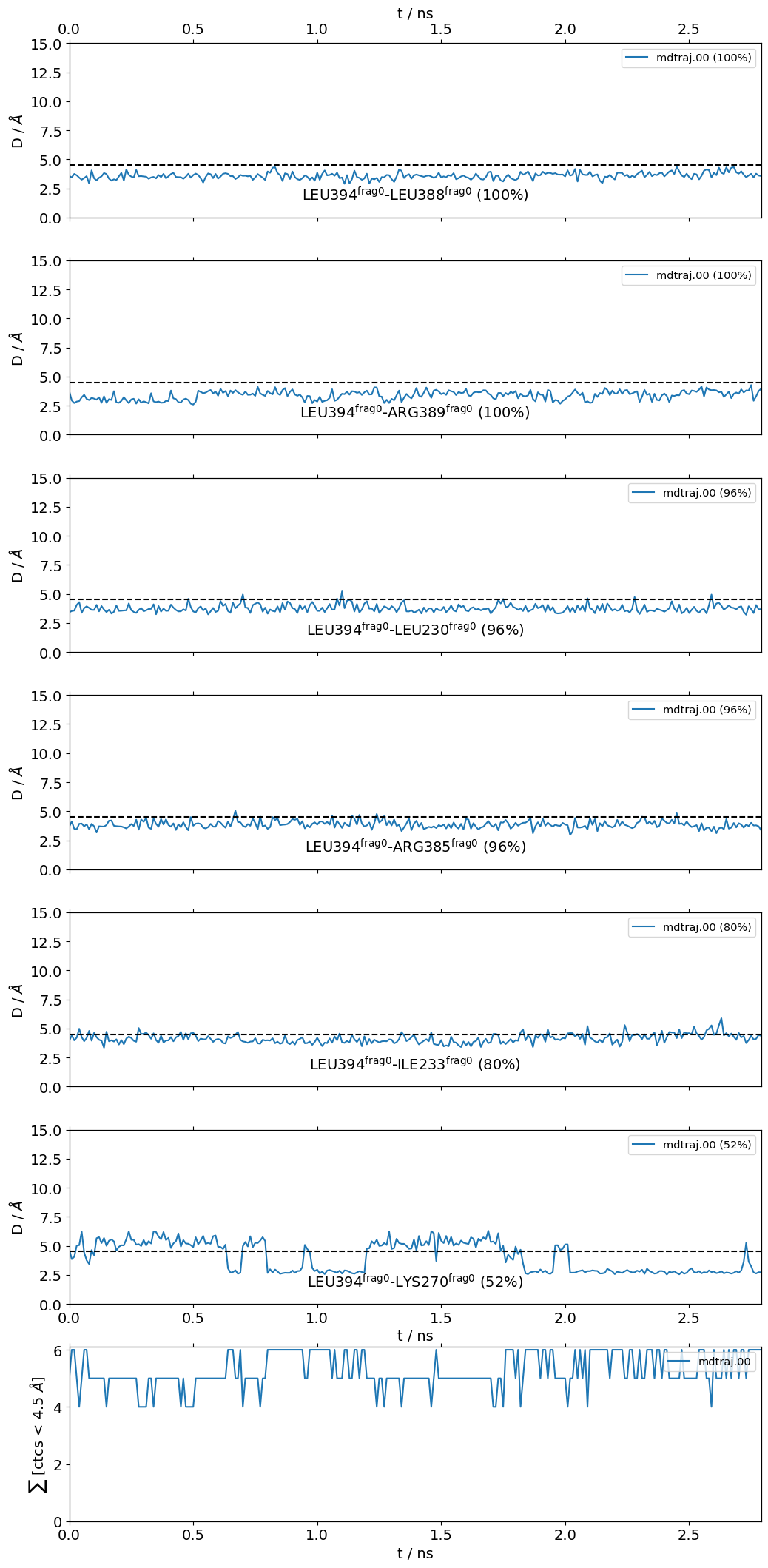
L394@frag0:
The following 6 contacts capture 5.26 (~97%) of the total frequency 5.43 (over 9 contacts with nonzero frequency at 4.50 Angstrom).
As orientation value, the first 6 ctcs already capture 90.0% of 5.43.
The 6-th contact has a frequency of 0.52.
   freq          label            residues  fragments   sum
1  1.00  L394@frag0 - L388@frag0  353 - 347    0 - 0   1.00
2  1.00  L394@frag0 - R389@frag0  353 - 348    0 - 0   2.00
3  0.97  L394@frag0 - L230@frag0  353 - 957    0 - 0   2.97
4  0.97  L394@frag0 - R385@frag0  353 - 344    0 - 0   3.94
5  0.80  L394@frag0 - I233@frag0  353 - 960    0 - 0   4.74
6  0.52  L394@frag0 - K270@frag0  353 - 972    0 - 0   5.26
The following files have been created:
./neighborhood.overall@4.5_Ang.pdf
./neighborhood.LEU394@frag0@4.5_Ang.dat
./neighborhood.LEU394@frag0.time_trace@4.5_Ang.pdf
neighborhoods is a dictionary keyed with residue indices and valued with a ContactGroup for each residue neighborhood.
ContactGroups are mdciao classes that allow the further manipulation of contact data, molecular information and much more. Check here to learn more about mdciao classes.
[3]:
neighborhoods[353]
[3]:
<mdciao.contacts.contacts.ContactGroup at 0x79d262074310>
Using Python Objects
Please note that in API mode, inputs can be objects, for example mdtraj Trajectories. So, before calling the next mdciao.cli method, we use mdtraj to load the trajectory from our files:
[4]:
import mdtraj as md
traj = md.load("mdciao_example/traj.xtc", top="mdciao_example/top.pdb")
traj
[4]:
<mdtraj.Trajectory with 280 frames, 8384 atoms, 1044 residues, and unitcells at 0x79d262370310>
And we repeat the above command using the traj object. Please note that we’re also using the no_disk option so that no files are written to disk, in case we’re only interested in working in memory.
[5]:
neighborhoods = mdciao.cli.residue_neighborhoods("L394",
                                                 traj,
                                                 fragments=None,
                                                 no_disk=True)
Will compute contact frequencies for (1 items):
<mdtraj.Trajectory with 280 frames, 8384 atoms, 1044 residues, and unitcells>
 with a stride of 1 frames
Using method 'None' these fragments were found
fragment 0 with   1044 AAs     LEU4 (   0) -   P0G395 (1043) (0) resSeq jumps

Will compute neighborhoods for the residues
L394
excluding 4 nearest neighbors

   residue      residx    fragment      resSeq
    LEU394         353           0         394

Performing a first pass on 1039 residue pairs to compute lower bounds on residue-residue distances via residue-COM distances:
Reduced to only 43 residue pairs for the computation of actual residue-residue distances:
L394@frag0:
The following 6 contacts capture 5.26 (~97%) of the total frequency 5.43 (over 9 contacts with nonzero frequency at 4.50 Angstrom).
As orientation value, the first 6 ctcs already capture 90.0% of 5.43.
The 6-th contact has a frequency of 0.52.
   freq          label            residues  fragments   sum
1  1.00  L394@frag0 - L388@frag0  353 - 347    0 - 0   1.00
2  1.00  L394@frag0 - R389@frag0  353 - 348    0 - 0   2.00
3  0.97  L394@frag0 - L230@frag0  353 - 957    0 - 0   2.97
4  0.97  L394@frag0 - R385@frag0  353 - 344    0 - 0   3.94
5  0.80  L394@frag0 - I233@frag0  353 - 960    0 - 0   4.74
6  0.52  L394@frag0 - K270@frag0  353 - 972    0 - 0   5.26
Now, the more elaborated CLI-command:
mdc_neighborhoods.py top.pdb traj.xtc -r L394 --GPCR adrb2_human --CGN gnas2_human -ni -at #ni: not interactive, at: show atom-types
We keep the no_disk option to avoid writing to disk, but you can change this if you want. Please note that some options do not carry exactly the same names as their CLI equivalents. E.g. ni in the CLI (= don’t be interactive) is now accept_guess in the API. These differences are needed for compatiblity with other methods, but might get unified in the future.
[6]:
neighborhoods = mdciao.cli.residue_neighborhoods("L394",
                                                 traj,
                                                 GPCR_UniProt="adrb2_human",
                                                 CGN_UniProt="gnas2_human",
                                                 accept_guess=True,
                                                 plot_atomtypes=True,
                                                 no_disk=True)
Will compute contact frequencies for (1 items):
<mdtraj.Trajectory with 280 frames, 8384 atoms, 1044 residues, and unitcells>
 with a stride of 1 frames
Using method 'lig_resSeq+' these fragments were found
fragment 0 with    354 AAs     LEU4 (   0) -   LEU394 (353 ) (0) resSeq jumps
fragment 1 with    340 AAs     GLN1 ( 354) -   ASN340 (693 ) (1)
fragment 2 with     66 AAs     ALA2 ( 694) -    PHE67 (759 ) (2)
fragment 3 with    283 AAs    GLU30 ( 760) -   LEU340 (1042) (3) resSeq jumps
fragment 4 with      1 AAs   P0G395 (1043) -   P0G395 (1043) (4)
No local file ./adrb2_human.xlsx found, checking online in
https://gpcrdb.org/services/residues/extended/adrb2_human ...done!
Please cite the following reference to the GPCRdb:
 * Kooistra et al, (2021) GPCRdb in 2021: Integrating GPCR sequence, structure and function
   Nucleic Acids Research 49, D335--D343
   https://doi.org/10.1093/nar/gkaa1080
For more information, call mdciao.nomenclature.references()
The GPCR-labels align best with fragments: [3] (first-last: GLU30-LEU340).

Mapping the GPCR fragments onto your topology:
 TM1  with     32 AAs    GLU30@1.29x29   ( 760) -    PHE61@1.60x60   (791 ) (TM1)
 ICL1 with      4 AAs    GLU62@12.48x48  ( 792) -    GLN65@12.51x51  (795 ) (ICL1)
 TM2  with     32 AAs    THR66@2.37x37   ( 796) -    LYS97@2.68x67   (827 ) (TM2)
 ECL1 with      4 AAs    MET98@23.49x49  ( 828) -   PHE101@23.52x52  (831 ) (ECL1)
 TM3  with     36 AAs   GLY102@3.21x21   ( 832) -   SER137@3.56x56   (867 ) (TM3)
 ICL2 with      8 AAs   PRO138@34.50x50  ( 868) -   LEU145@34.57x57  (875 ) (ICL2)
 TM4  with     27 AAs   THR146@4.38x38   ( 876) -   HIS172@4.64x64   (902 ) (TM4)
 ECL2 with     20 AAs   TRP173           ( 903) -   THR195           (922 ) (ECL2) resSeq jumps
 TM5  with     42 AAs   ASN196@5.35x36   ( 923) -   GLU237@5.76x76   (964 ) (TM5)
 ICL3 with      2 AAs   GLY238           ( 965) -   ARG239           (966 ) (ICL3)
 TM6  with     35 AAs   CYS265@6.27x27   ( 967) -   GLN299@6.61x61   (1001) (TM6)
 ECL3 with      4 AAs   ASP300           (1002) -   ILE303           (1005) (ECL3)
 TM7  with     25 AAs   ARG304@7.31x30   (1006) -   ARG328@7.55x55   (1030) (TM7)
 H8   with     12 AAs   SER329@8.47x47   (1031) -   LEU340@8.58x58   (1042) (H8)
No local file ./gnas2_human.xlsx found, checking online in
https://gpcrdb.org/services/residues/extended/gnas2_human ...done!
Please cite the following reference to the GPCRdb:
 * Kooistra et al, (2021) GPCRdb in 2021: Integrating GPCR sequence, structure and function
   Nucleic Acids Research 49, D335--D343
   https://doi.org/10.1093/nar/gkaa1080
Please cite the following reference to the CGN nomenclature:
 * Flock et al, (2015) Universal allosteric mechanism for G$\alpha$ activation by GPCRs
   Nature 2015 524:7564 524, 173--179
   https://doi.org/10.1038/nature14663
For more information, call mdciao.nomenclature.references()
The CGN-labels align best with fragments: [0] (first-last: LEU4-LEU394).

Mapping the CGN fragments onto your topology:
 G.HN   with     33 AAs     LEU4@G.HN.10   (   0) -    VAL36@G.HN.53   (32  ) (G.HN)
 G.hns1 with      3 AAs    TYR37@G.hns1.01 (  33) -    ALA39@G.hns1.03 (35  ) (G.hns1)
 G.S1   with      7 AAs    THR40@G.S1.01   (  36) -    LEU46@G.S1.07   (42  ) (G.S1)
 G.s1h1 with      6 AAs    GLY47@G.s1h1.01 (  43) -    GLY52@G.s1h1.06 (48  ) (G.s1h1)
 G.H1   with      7 AAs    LYS53@G.H1.01   (  49) -    GLN59@G.H1.07   (55  ) (G.H1)
 H.HA   with     26 AAs    LYS88@H.HA.04   (  56) -   LEU113@H.HA.29   (81  ) (H.HA)
 H.hahb with      9 AAs   VAL114@H.hahb.01 (  82) -   PRO122@H.hahb.09 (90  ) (H.hahb)
 H.HB   with     14 AAs   GLU123@H.HB.01   (  91) -   ASN136@H.HB.14   (104 ) (H.HB)
 H.hbhc with      7 AAs   VAL137@H.hbhc.01 ( 105) -   PRO143@H.hbhc.15 (111 ) (H.hbhc)
 H.HC   with     12 AAs   PRO144@H.HC.01   ( 112) -   GLU155@H.HC.12   (123 ) (H.HC)
 H.hchd with      1 AAs   ASP156@H.hchd.01 ( 124) -   ASP156@H.hchd.01 (124 ) (H.hchd)
 H.HD   with     12 AAs   GLU157@H.HD.01   ( 125) -   GLU168@H.HD.12   (136 ) (H.HD)
 H.hdhe with      5 AAs   TYR169@H.hdhe.01 ( 137) -   ASP173@H.hdhe.05 (141 ) (H.hdhe)
 H.HE   with     13 AAs   CYS174@H.HE.01   ( 142) -   LYS186@H.HE.13   (154 ) (H.HE)
 H.hehf with      7 AAs   GLN187@H.hehf.01 ( 155) -   SER193@H.hehf.07 (161 ) (H.hehf)
 H.HF   with      6 AAs   ASP194@H.HF.01   ( 162) -   ARG199@H.HF.06   (167 ) (H.HF)
 G.hfs2 with      5 AAs   CYS200@G.hfs2.01 ( 168) -   GLY206@G.hfs2.07 (172 ) (G.hfs2) resSeq jumps
 G.S2   with      8 AAs   ILE207@G.S2.01   ( 173) -   VAL214@G.S2.08   (180 ) (G.S2)
 G.s2s3 with      2 AAs   ASP215@G.s2s3.01 ( 181) -   LYS216@G.s2s3.02 (182 ) (G.s2s3)
 G.S3   with      8 AAs   VAL217@G.S3.01   ( 183) -   VAL224@G.S3.08   (190 ) (G.S3)
 G.s3h2 with      3 AAs   GLY225@G.s3h2.01 ( 191) -   GLN227@G.s3h2.03 (193 ) (G.s3h2)
 G.H2   with     10 AAs   ARG228@G.H2.01   ( 194) -   CYS237@G.H2.10   (203 ) (G.H2)
 G.h2s4 with      5 AAs   PHE238@G.h2s4.01 ( 204) -   THR242@G.h2s4.05 (208 ) (G.h2s4)
 G.S4   with      7 AAs   ALA243@G.S4.01   ( 209) -   ALA249@G.S4.07   (215 ) (G.S4)
 G.s4h3 with      8 AAs   SER250@G.s4h3.01 ( 216) -   ASN264@G.s4h3.15 (223 ) (G.s4h3) resSeq jumps
 G.H3   with     18 AAs   ARG265@G.H3.01   ( 224) -   LEU282@G.H3.18   (241 ) (G.H3)
 G.h3s5 with      3 AAs   ARG283@G.h3s5.01 ( 242) -   ILE285@G.h3s5.03 (244 ) (G.h3s5)
 G.S5   with      7 AAs   SER286@G.S5.01   ( 245) -   ASN292@G.S5.07   (251 ) (G.S5)
 G.s5hg with      1 AAs   LYS293@G.s5hg.01 ( 252) -   LYS293@G.s5hg.01 (252 ) (G.s5hg)
 G.HG   with     17 AAs   GLN294@G.HG.01   ( 253) -   ASP310@G.HG.17   (269 ) (G.HG)
 G.hgh4 with     21 AAs   TYR311@G.hgh4.01 ( 270) -   ASP331@G.hgh4.21 (290 ) (G.hgh4)
 G.H4   with     16 AAs   PRO332@G.H4.01   ( 291) -   ARG347@G.H4.17   (306 ) (G.H4)
 G.h4s6 with     11 AAs   ILE348@G.h4s6.01 ( 307) -   TYR358@G.h4s6.20 (317 ) (G.h4s6)
 G.S6   with      5 AAs   CYS359@G.S6.01   ( 318) -   PHE363@G.S6.05   (322 ) (G.S6)
 G.s6h5 with      5 AAs   THR364@G.s6h5.01 ( 323) -   ASP368@G.s6h5.05 (327 ) (G.s6h5)
 G.H5   with     26 AAs   THR369@G.H5.01   ( 328) -   LEU394@G.H5.26   (353 ) (G.H5)

Will compute neighborhoods for the residues
L394
excluding 4 nearest neighbors

   residue      residx    fragment      resSeq        GPCR         CGN
    LEU394         353           0         394        None     G.H5.26

Performing a first pass on 1039 residue pairs to compute lower bounds on residue-residue distances via residue-COM distances:
Reduced to only 43 residue pairs for the computation of actual residue-residue distances:
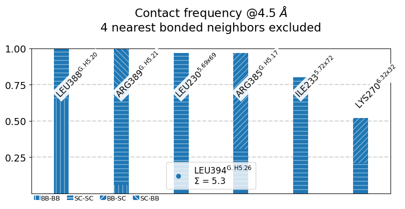
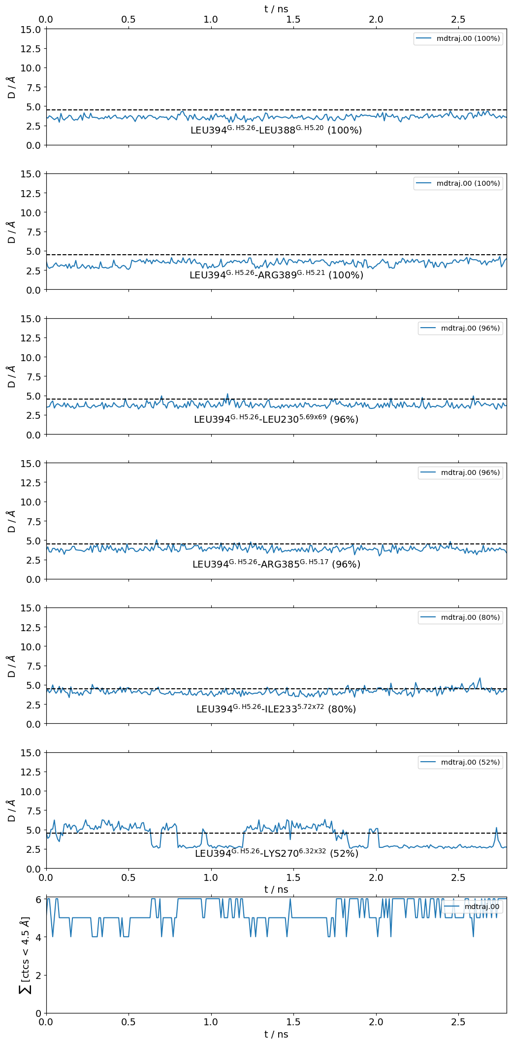
L394@G.H5.26:
The following 6 contacts capture 5.26 (~97%) of the total frequency 5.43 (over 9 contacts with nonzero frequency at 4.50 Angstrom).
As orientation value, the first 6 ctcs already capture 90.0% of 5.43.
The 6-th contact has a frequency of 0.52.
   freq            label              residues  fragments   sum
1  1.00  L394@G.H5.26 - L388@G.H5.20  353 - 347    0 - 0   1.00
2  1.00  L394@G.H5.26 - R389@G.H5.21  353 - 348    0 - 0   2.00
3  0.97  L394@G.H5.26 - L230@5.69x69  353 - 957    0 - 3   2.97
4  0.97  L394@G.H5.26 - R385@G.H5.17  353 - 344    0 - 0   3.94
5  0.80  L394@G.H5.26 - I233@5.72x72  353 - 960    0 - 3   4.74
6  0.52  L394@G.H5.26 - K270@6.32x32  353 - 972    0 - 3   5.26
Consensus Nomenclature: GPCR and/or CGN
Above, we declared our intention to use GPCR consensus nomenclature and Common G-alpha Numbering (CGN) by passing the descriptor strings GPCR_UniProt="adrb2_human" or CGN_UniProt="gnas2_human", respectively, to contact the online databases, in particular the
GPCRdb, Kooistra et al, (2021) GPCRdb in 2021: Integrating GPCR sequence, structure and function, Nucleic Acids Research 49, D335–D343, https://doi.org/10.1093/nar/gkaa1080
For that retrieval and handling of these labels, we use the module mdciao.nomenclature, which offers classes and other helper functions to deal with the nomenclature. An overview of the relevant references is contained in the module’s
documentation as well as in the documentation of each class, e.g. here.
Additionally, you can use mdciao.nomenclature.references to print all relevant nomenclature references:
[7]:
mdciao.nomenclature.references()
mdciao.nomenclature functions thanks to these online databases. Please cite them if you use this module:
 * Kooistra et al, (2021) GPCRdb in 2021: Integrating GPCR sequence, structure and function
   Nucleic Acids Research 49, D335--D343
   https://doi.org/10.1093/nar/gkaa1080
 * Berman et al, (2000) The Protein Data Bank
   Nucleic Acids Research 28, 235--242
   https://doi.org/10.1093/NAR/28.1.235
 * Flock et al, (2015) Universal allosteric mechanism for G$\alpha$ activation by GPCRs
   Nature 2015 524:7564 524, 173--179
   https://doi.org/10.1038/nature14663
 * Kanev et al, (2021) KLIFS: an overhaul after the first 5 years of supporting kinase research
   Nucleic Acids Research 49, D562--D569
   https://doi.org/10.1093/NAR/GKAA895

Additionally, depending on the chosen nomenclature type, you should cite:
 * Structure based GPCR notation
   - Isberg et al, (2015) Generic GPCR residue numbers - Aligning topology maps while minding the gaps
     Trends in Pharmacological Sciences 36, 22--31
     https://doi.org/10.1016/j.tips.2014.11.001
   - Isberg et al, (2016) GPCRdb: An information system for G protein-coupled receptors
     Nucleic Acids Research 44, D356--D364
     https://doi.org/10.1093/nar/gkv1178
 * Sequence based GPCR schemes:
   - Wootten et al, (2013) Polar transmembrane interactions drive formation of ligand-specific and signal
     pathway-biased family B G protein-coupled receptor conformations
     Proceedings of the National Academy of Sciences of the United States of America 110, 5211--5216
     https://doi.org/10.1073/pnas.1221585110
   - Pin et al, (2003) Evolution, structure, and activation mechanism of family 3/C G-protein-coupled
     receptors
     Pharmacology and Therapeutics 98, 325--354
     https://doi.org/10.1016/S0163-7258(03)00038-X
   - Wu et al, (2014) Structure of a class C GPCR metabotropic glutamate receptor 1 bound to an
     allosteric modulator
     Science 344, 58--64
     https://doi.org/10.1126/science.1249489
   - Oliveira et al, (1993) A common motif in G-protein-coupled seven transmembrane helix receptors
     Journal of Computer-Aided Molecular Design 7, 649--658
     https://doi.org/10.1007/BF00125323
   - Baldwin et al, (1993) The probable arrangement of the helices in G protein-coupled receptors.
     The EMBO Journal 12, 1693--1703
     https://doi.org/10.1002/J.1460-2075.1993.TB05814.X
   - Baldwin et al, (1997) An alpha-carbon template for the transmembrane helices in the rhodopsin family
     of G-protein-coupled receptors
     Journal of Molecular Biology 272, 144--164
     https://doi.org/10.1006/jmbi.1997.1240
   - Schwartz et al, (1994) Locating ligand-binding sites in 7tm receptors by protein engineering
     Current Opinion in Biotechnology 5, 434--444
     https://doi.org/10.1016/0958-1669(94)90054-X
   - Schwartz et al, (1995) Molecular mechanism of action of non-peptide ligands for peptide receptors
     Current Pharmaceutical Design 1, 325--342
 * KLIFS 85 ligand binding site residues of kinases
   - Van Linden et al, (2014) KLIFS: A knowledge-based structural database to navigate kinase-ligand
     interaction space
     Journal of Medicinal Chemistry 57, 249--277
     https://doi.org/10.1021/JM400378W
   - Kooistra et al, (2016) KLIFS: a structural kinase-ligand interaction database
     Nucleic Acids Research 44, D365--D371
     https://doi.org/10.1093/NAR/GKV1082
   - Kanev et al, (2021) KLIFS: an overhaul after the first 5 years of supporting kinase research
     Nucleic Acids Research 49, D562--D569
     https://doi.org/10.1093/NAR/GKAA895

You can find all these references distributed as BibTex file distributed with mdciao here
 * /media/perezheg/363d9114-5236-44c6-be82-5d40142f32e71/home/perezheg/Programs/mdciao/tests/data/nomenclature/nomenclature.bib
The nomenclature classes produce standalone objects, and can do much more than just be inputs to mdciao.cli methods. As with any Python class, you can learn a lot about its methods and attributes by using the tab autocompletion feature of IPython. Or you can check here for more mdciao docs.
Since we’ll be using these labels more than once in the notebook, instead of using the network each time, we can have them as Python objects in memory. Alternatively, it’s possible to save the labeling data locally after the first database query. This allows for inspection and re-use of the retrieved data outside the notebook (in a spreadsheet, for example).
[8]:
from mdciao import nomenclature
GPCR = nomenclature.LabelerGPCR("adrb2_human",
                            #write_to_disk=True
                           )
CGN = nomenclature.LabelerCGN("gnas2_human",
                             # write_to_disk=True
                             )
No local file ./adrb2_human.xlsx found, checking online in
https://gpcrdb.org/services/residues/extended/adrb2_human ...done!
Please cite the following reference to the GPCRdb:
 * Kooistra et al, (2021) GPCRdb in 2021: Integrating GPCR sequence, structure and function
   Nucleic Acids Research 49, D335--D343
   https://doi.org/10.1093/nar/gkaa1080
For more information, call mdciao.nomenclature.references()
No local file ./gnas2_human.xlsx found, checking online in
https://gpcrdb.org/services/residues/extended/gnas2_human ...done!
Please cite the following reference to the GPCRdb:
 * Kooistra et al, (2021) GPCRdb in 2021: Integrating GPCR sequence, structure and function
   Nucleic Acids Research 49, D335--D343
   https://doi.org/10.1093/nar/gkaa1080
Please cite the following reference to the CGN nomenclature:
 * Flock et al, (2015) Universal allosteric mechanism for G$\alpha$ activation by GPCRs
   Nature 2015 524:7564 524, 173--179
   https://doi.org/10.1038/nature14663
For more information, call mdciao.nomenclature.references()
Residue Selection
Now, we can play around with residue selection, replicating the CLI-command:
mdc_residues.py GLU*,P0G,380-394,G.HN.* top.pdb --GPCR adrb2_human --CGN gnas2_human -ni
Check the docs here to check the output values res_idxs_list,fragments, and consensus_maps, although most of the useful output is written out.
Please note that we’re now using mdciao.nomenclature classes directly as inputs (GPCR and CGN), speeding up the method by avoiding queries over the network.
[9]:
res_idxs_list, fragments, consensus_maps = mdciao.cli.residue_selection(
    "GLU*,P0G,380-394,G.HN.*",
    traj,
    GPCR_UniProt=GPCR,
    CGN_UniProt=CGN,
    accept_guess=True)
Using method 'lig_resSeq+' these fragments were found
fragment 0 with 354 AAs LEU4 ( 0) - LEU394 (353 ) (0) resSeq jumps
fragment 1 with 340 AAs GLN1 ( 354) - ASN340 (693 ) (1)
fragment 2 with 66 AAs ALA2 ( 694) - PHE67 (759 ) (2)
fragment 3 with 283 AAs GLU30 ( 760) - LEU340 (1042) (3) resSeq jumps
fragment 4 with 1 AAs P0G395 (1043) - P0G395 (1043) (4)
The GPCR-labels align best with fragments: [3] (first-last: GLU30-LEU340).
Mapping the GPCR fragments onto your topology:
TM1 with 32 AAs GLU30@1.29x29 ( 760) - PHE61@1.60x60 (791 ) (TM1)
ICL1 with 4 AAs GLU62@12.48x48 ( 792) - GLN65@12.51x51 (795 ) (ICL1)
TM2 with 32 AAs THR66@2.37x37 ( 796) - LYS97@2.68x67 (827 ) (TM2)
ECL1 with 4 AAs MET98@23.49x49 ( 828) - PHE101@23.52x52 (831 ) (ECL1)
TM3 with 36 AAs GLY102@3.21x21 ( 832) - SER137@3.56x56 (867 ) (TM3)
ICL2 with 8 AAs PRO138@34.50x50 ( 868) - LEU145@34.57x57 (875 ) (ICL2)
TM4 with 27 AAs THR146@4.38x38 ( 876) - HIS172@4.64x64 (902 ) (TM4)
ECL2 with 20 AAs TRP173 ( 903) - THR195 (922 ) (ECL2) resSeq jumps
TM5 with 42 AAs ASN196@5.35x36 ( 923) - GLU237@5.76x76 (964 ) (TM5)
ICL3 with 2 AAs GLY238 ( 965) - ARG239 (966 ) (ICL3)
TM6 with 35 AAs CYS265@6.27x27 ( 967) - GLN299@6.61x61 (1001) (TM6)
ECL3 with 4 AAs ASP300 (1002) - ILE303 (1005) (ECL3)
TM7 with 25 AAs ARG304@7.31x30 (1006) - ARG328@7.55x55 (1030) (TM7)
H8 with 12 AAs SER329@8.47x47 (1031) - LEU340@8.58x58 (1042) (H8)
The CGN-labels align best with fragments: [0] (first-last: LEU4-LEU394).
Mapping the CGN fragments onto your topology:
G.HN with 33 AAs LEU4@G.HN.10 ( 0) - VAL36@G.HN.53 (32 ) (G.HN)
G.hns1 with 3 AAs TYR37@G.hns1.01 ( 33) - ALA39@G.hns1.03 (35 ) (G.hns1)
G.S1 with 7 AAs THR40@G.S1.01 ( 36) - LEU46@G.S1.07 (42 ) (G.S1)
G.s1h1 with 6 AAs GLY47@G.s1h1.01 ( 43) - GLY52@G.s1h1.06 (48 ) (G.s1h1)
G.H1 with 7 AAs LYS53@G.H1.01 ( 49) - GLN59@G.H1.07 (55 ) (G.H1)
H.HA with 26 AAs LYS88@H.HA.04 ( 56) - LEU113@H.HA.29 (81 ) (H.HA)
H.hahb with 9 AAs VAL114@H.hahb.01 ( 82) - PRO122@H.hahb.09 (90 ) (H.hahb)
H.HB with 14 AAs GLU123@H.HB.01 ( 91) - ASN136@H.HB.14 (104 ) (H.HB)
H.hbhc with 7 AAs VAL137@H.hbhc.01 ( 105) - PRO143@H.hbhc.15 (111 ) (H.hbhc)
H.HC with 12 AAs PRO144@H.HC.01 ( 112) - GLU155@H.HC.12 (123 ) (H.HC)
H.hchd with 1 AAs ASP156@H.hchd.01 ( 124) - ASP156@H.hchd.01 (124 ) (H.hchd)
H.HD with 12 AAs GLU157@H.HD.01 ( 125) - GLU168@H.HD.12 (136 ) (H.HD)
H.hdhe with 5 AAs TYR169@H.hdhe.01 ( 137) - ASP173@H.hdhe.05 (141 ) (H.hdhe)
H.HE with 13 AAs CYS174@H.HE.01 ( 142) - LYS186@H.HE.13 (154 ) (H.HE)
H.hehf with 7 AAs GLN187@H.hehf.01 ( 155) - SER193@H.hehf.07 (161 ) (H.hehf)
H.HF with 6 AAs ASP194@H.HF.01 ( 162) - ARG199@H.HF.06 (167 ) (H.HF)
G.hfs2 with 5 AAs CYS200@G.hfs2.01 ( 168) - GLY206@G.hfs2.07 (172 ) (G.hfs2) resSeq jumps
G.S2 with 8 AAs ILE207@G.S2.01 ( 173) - VAL214@G.S2.08 (180 ) (G.S2)
G.s2s3 with 2 AAs ASP215@G.s2s3.01 ( 181) - LYS216@G.s2s3.02 (182 ) (G.s2s3)
G.S3 with 8 AAs VAL217@G.S3.01 ( 183) - VAL224@G.S3.08 (190 ) (G.S3)
G.s3h2 with 3 AAs GLY225@G.s3h2.01 ( 191) - GLN227@G.s3h2.03 (193 ) (G.s3h2)
G.H2 with 10 AAs ARG228@G.H2.01 ( 194) - CYS237@G.H2.10 (203 ) (G.H2)
G.h2s4 with 5 AAs PHE238@G.h2s4.01 ( 204) - THR242@G.h2s4.05 (208 ) (G.h2s4)
G.S4 with 7 AAs ALA243@G.S4.01 ( 209) - ALA249@G.S4.07 (215 ) (G.S4)
G.s4h3 with 8 AAs SER250@G.s4h3.01 ( 216) - ASN264@G.s4h3.15 (223 ) (G.s4h3) resSeq jumps
G.H3 with 18 AAs ARG265@G.H3.01 ( 224) - LEU282@G.H3.18 (241 ) (G.H3)
G.h3s5 with 3 AAs ARG283@G.h3s5.01 ( 242) - ILE285@G.h3s5.03 (244 ) (G.h3s5)
G.S5 with 7 AAs SER286@G.S5.01 ( 245) - ASN292@G.S5.07 (251 ) (G.S5)
G.s5hg with 1 AAs LYS293@G.s5hg.01 ( 252) - LYS293@G.s5hg.01 (252 ) (G.s5hg)
G.HG with 17 AAs GLN294@G.HG.01 ( 253) - ASP310@G.HG.17 (269 ) (G.HG)
G.hgh4 with 21 AAs TYR311@G.hgh4.01 ( 270) - ASP331@G.hgh4.21 (290 ) (G.hgh4)
G.H4 with 16 AAs PRO332@G.H4.01 ( 291) - ARG347@G.H4.17 (306 ) (G.H4)
G.h4s6 with 11 AAs ILE348@G.h4s6.01 ( 307) - TYR358@G.h4s6.20 (317 ) (G.h4s6)
G.S6 with 5 AAs CYS359@G.S6.01 ( 318) - PHE363@G.S6.05 (322 ) (G.S6)
G.s6h5 with 5 AAs THR364@G.s6h5.01 ( 323) - ASP368@G.s6h5.05 (327 ) (G.s6h5)
G.H5 with 26 AAs THR369@G.H5.01 ( 328) - LEU394@G.H5.26 (353 ) (G.H5)
0.0) P0G395 in fragment 4 with residue index 1043
0.0) ARG380 in fragment 0 with residue index 339 ( CGN: ARG380@G.H5.12)
0.0) LEU394 in fragment 0 with residue index 353 ( CGN: LEU394@G.H5.26)
Your selection 'GLU*,P0G,380-394,G.HN.*' yields:
residue residx fragment resSeq GPCR CGN
GLU10 6 0 10 None G.HN.27
GLU15 11 0 15 None G.HN.32
GLU16 12 0 16 None G.HN.33
GLU21 17 0 21 None G.HN.38
GLU27 23 0 27 None G.HN.44
GLU50 46 0 50 None G.s1h1.04
GLU101 69 0 101 None H.HA.17
GLU104 72 0 104 None H.HA.20
GLU118 86 0 118 None H.hahb.05
GLU123 91 0 123 None H.HB.01
GLU145 113 0 145 None H.HC.02
GLU148 116 0 148 None H.HC.05
GLU155 123 0 155 None H.HC.12
GLU157 125 0 157 None H.HD.01
GLU164 132 0 164 None H.HD.08
GLU168 136 0 168 None H.HD.12
GLU209 175 0 209 None G.S2.03
GLU230 196 0 230 None G.H2.03
GLU268 227 0 268 None G.H3.04
GLU299 258 0 299 None G.HG.06
GLU309 268 0 309 None G.HG.16
GLU314 273 0 314 None G.hgh4.04
GLU322 281 0 322 None G.hgh4.12
GLU327 286 0 327 None G.hgh4.17
GLU330 289 0 330 None G.hgh4.20
GLU344 303 0 344 None G.H4.14
GLU370 329 0 370 None G.H5.02
GLU392 351 0 392 None G.H5.24
GLU3 356 1 3 None None
GLU10 363 1 10 None None
GLU12 365 1 12 None None
GLU130 483 1 130 None None
GLU138 491 1 138 None None
GLU172 525 1 172 None None
GLU215 568 1 215 None None
GLU226 579 1 226 None None
GLU260 613 1 260 None None
GLU17 709 2 17 None None
GLU22 714 2 22 None None
GLU42 734 2 42 None None
GLU47 739 2 47 None None
GLU58 750 2 58 None None
GLU63 755 2 63 None None
GLU30 760 3 30 1.29x29 None
GLU62 792 3 62 12.48x48 None
GLU107 837 3 107 3.26x26 None
GLU122 852 3 122 3.41x41 None
GLU180 907 3 180 None None
GLU188 915 3 188 None None
GLU225 952 3 225 5.64x64 None
GLU237 964 3 237 5.76x76 None
GLU268 970 3 268 6.30x30 None
GLU306 1008 3 306 7.33x32 None
GLU338 1040 3 338 8.56x56 None
P0G395 1043 4 395 None None
ARG380 339 0 380 None G.H5.12
ASP381 340 0 381 None G.H5.13
ILE382 341 0 382 None G.H5.14
ILE383 342 0 383 None G.H5.15
GLN384 343 0 384 None G.H5.16
ARG385 344 0 385 None G.H5.17
MET386 345 0 386 None G.H5.18
HIS387 346 0 387 None G.H5.19
LEU388 347 0 388 None G.H5.20
ARG389 348 0 389 None G.H5.21
GLN390 349 0 390 None G.H5.22
TYR391 350 0 391 None G.H5.23
LEU393 352 0 393 None G.H5.25
LEU394 353 0 394 None G.H5.26
LEU4 0 0 4 None G.HN.10
GLY5 1 0 5 None G.HN.11
ASN6 2 0 6 None G.HN.22
SER7 3 0 7 None G.HN.23
LYS8 4 0 8 None G.HN.24
THR9 5 0 9 None G.HN.26
ASP11 7 0 11 None G.HN.28
GLN12 8 0 12 None G.HN.29
ARG13 9 0 13 None G.HN.30
ASN14 10 0 14 None G.HN.31
LYS17 13 0 17 None G.HN.34
ALA18 14 0 18 None G.HN.35
GLN19 15 0 19 None G.HN.36
ARG20 16 0 20 None G.HN.37
ALA22 18 0 22 None G.HN.39
ASN23 19 0 23 None G.HN.40
LYS24 20 0 24 None G.HN.41
LYS25 21 0 25 None G.HN.42
ILE26 22 0 26 None G.HN.43
LYS28 24 0 28 None G.HN.45
GLN29 25 0 29 None G.HN.46
LEU30 26 0 30 None G.HN.47
GLN31 27 0 31 None G.HN.48
LYS32 28 0 32 None G.HN.49
ASP33 29 0 33 None G.HN.50
LYS34 30 0 34 None G.HN.51
GLN35 31 0 35 None G.HN.52
VAL36 32 0 36 None G.HN.53
PDB Queries
Now we grab a structure directly from the PDB, replicating the CLI command:
mdc_pdb.py 3SN6 -o 3SN6.gro
by using mdciao.cli.pdb. Check here or use the inline docstring for more info. Please note that we’re not storing the retrived structure on disk, but rather having it in memory as an mdtraj.Trajectory:
[10]:
xray3SN6= mdciao.cli.pdb("3SN6")
xray3SN6
Checking https://files.rcsb.org/download/3SN6.pdb ...Please cite the following 3rd party publication:
 * Crystal structure of the beta2 adrenergic receptor-Gs protein complex
   Rasmussen, S.G. et al., Nature 2011
   https://doi.org/10.1038/nature10361
[10]:
<mdtraj.Trajectory with 1 frames, 10274 atoms, 1319 residues, and unitcells at 0x79d2b4fa4310>
Now we can use the awesome nglviewer to 3D-visualize the freshly grabbed structure inside the notebook.
We need to import the module first, which needs to be installed in your Python environment. If you don’t we recommend you install it via pip:
pip install nglview
jupyter-nbextension enable nglview --py --sys-prefix
If you don’t feel like installing now, you can continue use the notebook.
[11]:
try:
    import nglview
    iwd = nglview.show_mdtraj(xray3SN6)
except ImportError:
    iwd = None
iwd
Fragmentation Heuristics
Now we go to fragmentation heuristics, replicating the CLI command:
mdc_fragments.py 3SN6.gro
but with the object xray3SN6 (the .gro-file comes below) and by using the cli.fragments method. Check here or the inline docstring for more info. Also note that cli.fragments simply wraps around mdciao.fragments.get_fragments, and
you can use that method (or others in mdciao.fragments) directly.
[12]:
frags= mdciao.cli.fragment_overview(xray3SN6.top)
Auto-detected fragments with method 'chains'
fragment      0 with    349 AAs     THR9 (   0) -   LEU394 (348 ) (0) resSeq jumps
fragment      1 with    340 AAs     GLN1 ( 349) -   ASN340 (688 ) (1)
fragment      2 with     58 AAs     ASN5 ( 689) -    ARG62 (746 ) (2)
fragment      3 with    443 AAs  ASN1002 ( 747) -   CYS341 (1189) (3) resSeq jumps
fragment      4 with    128 AAs     GLN1 (1190) -   SER128 (1317) (4)
fragment      5 with      1 AAs  P0G1601 (1318) -  P0G1601 (1318) (5)

Auto-detected fragments with method 'resSeq'
fragment      0 with     51 AAs     THR9 (   0) -    GLN59 (50  ) (0)
fragment      1 with    115 AAs    LYS88 (  51) -   VAL202 (165 ) (1)
fragment      2 with     51 AAs   SER205 ( 166) -   MET255 (216 ) (2)
fragment      3 with    132 AAs   THR263 ( 217) -   LEU394 (348 ) (3)
fragment      4 with    340 AAs     GLN1 ( 349) -   ASN340 (688 ) (4)
fragment      5 with     58 AAs     ASN5 ( 689) -    ARG62 (746 ) (5)
fragment      6 with    159 AAs  ASN1002 ( 747) -  ALA1160 (905 ) (6)
fragment      7 with    146 AAs    GLU30 ( 906) -   ARG175 (1051) (7)
fragment      8 with     61 AAs   GLN179 (1052) -   ARG239 (1112) (8)
fragment      9 with     77 AAs   CYS265 (1113) -   CYS341 (1189) (9)
fragment     10 with    128 AAs     GLN1 (1190) -   SER128 (1317) (10)
fragment     11 with      1 AAs  P0G1601 (1318) -  P0G1601 (1318) (11)

Auto-detected fragments with method 'resSeq+'
fragment      0 with    349 AAs     THR9 (   0) -   LEU394 (348 ) (0) resSeq jumps
fragment      1 with    340 AAs     GLN1 ( 349) -   ASN340 (688 ) (1)
fragment      2 with     58 AAs     ASN5 ( 689) -    ARG62 (746 ) (2)
fragment      3 with    159 AAs  ASN1002 ( 747) -  ALA1160 (905 ) (3)
fragment      4 with    284 AAs    GLU30 ( 906) -   CYS341 (1189) (4) resSeq jumps
fragment      5 with    128 AAs     GLN1 (1190) -   SER128 (1317) (5)
fragment      6 with      1 AAs  P0G1601 (1318) -  P0G1601 (1318) (6)

Auto-detected fragments with method 'lig_resSeq+'
fragment      0 with    349 AAs     THR9 (   0) -   LEU394 (348 ) (0) resSeq jumps
fragment      1 with    340 AAs     GLN1 ( 349) -   ASN340 (688 ) (1)
fragment      2 with     58 AAs     ASN5 ( 689) -    ARG62 (746 ) (2)
fragment      3 with    159 AAs  ASN1002 ( 747) -  ALA1160 (905 ) (3)
fragment      4 with    284 AAs    GLU30 ( 906) -   CYS341 (1189) (4) resSeq jumps
fragment      5 with    128 AAs     GLN1 (1190) -   SER128 (1317) (5)
fragment      6 with      1 AAs  P0G1601 (1318) -  P0G1601 (1318) (6)

Auto-detected fragments with method 'bonds'
fragment      0 with    349 AAs     THR9 (   0) -   LEU394 (348 ) (0) resSeq jumps
fragment      1 with    340 AAs     GLN1 ( 349) -   ASN340 (688 ) (1)
fragment      2 with     58 AAs     ASN5 ( 689) -    ARG62 (746 ) (2)
fragment      3 with    443 AAs  ASN1002 ( 747) -   CYS341 (1189) (3) resSeq jumps
fragment      4 with    128 AAs     GLN1 (1190) -   SER128 (1317) (4)
fragment      5 with      1 AAs  P0G1601 (1318) -  P0G1601 (1318) (5)

Auto-detected fragments with method 'resSeq_bonds'
fragment      0 with     51 AAs     THR9 (   0) -    GLN59 (50  ) (0)
fragment      1 with    115 AAs    LYS88 (  51) -   VAL202 (165 ) (1)
fragment      2 with     51 AAs   SER205 ( 166) -   MET255 (216 ) (2)
fragment      3 with    132 AAs   THR263 ( 217) -   LEU394 (348 ) (3)
fragment      4 with    340 AAs     GLN1 ( 349) -   ASN340 (688 ) (4)
fragment      5 with     58 AAs     ASN5 ( 689) -    ARG62 (746 ) (5)
fragment      6 with    159 AAs  ASN1002 ( 747) -  ALA1160 (905 ) (6)
fragment      7 with    146 AAs    GLU30 ( 906) -   ARG175 (1051) (7)
fragment      8 with     61 AAs   GLN179 (1052) -   ARG239 (1112) (8)
fragment      9 with     77 AAs   CYS265 (1113) -   CYS341 (1189) (9)
fragment     10 with    128 AAs     GLN1 (1190) -   SER128 (1317) (10)
fragment     11 with      1 AAs  P0G1601 (1318) -  P0G1601 (1318) (11)

Auto-detected fragments with method 'None'
fragment      0 with   1319 AAs     THR9 (   0) -  P0G1601 (1318) (0) resSeq jumps
This call iterates through all available heuristics on the mdtrajTopology, arriving at different definitions of molecular fragments. They are all returned as a dictionary:
[13]:
frags.keys()
[13]:
dict_keys(['chains', 'resSeq', 'resSeq+', 'lig_resSeq+', 'bonds', 'resSeq_bonds', 'None'])
Please note that since xray3SN6 comes from the PDB directly, it contains chain descriptors, s.t. the method chains (first one) can simply list the chain information encoded into the PDB, which you can check here:
Auto-detected fragments with method 'chains'
fragment      0 with    349 AAs     THR9 (     0) -   LEU394 (348   ) (0)  resSeq jumps
fragment      1 with    340 AAs     GLN1 (   349) -   ASN340 (688   ) (1)
fragment      2 with     58 AAs     ASN5 (   689) -    ARG62 (746   ) (2)
fragment      3 with    443 AAs  ASN1002 (   747) -   CYS341 (1189  ) (3)  resSeq jumps
fragment      4 with    128 AAs     GLN1 (  1190) -   SER128 (1317  ) (4)
fragment      5 with      1 AAs  P0G1601 (  1318) -  P0G1601 (1318  ) (5)       5 with    1 AAs  P0G1601           (1318) -  P0G1601           (1318) (5)
These fragments are:
G-protein \(\alpha\) sub-unit
G-protein \(\beta\) sub-unit
G-protein \(\gamma\) sub-unit
\(\beta_2\) adrenergic receptor, together with the bacteriophage T4 lysozyme as N-terminus
VHH nanobody
Ligand P0G
However, we loose that chain information if we store the structure as .gro, which doesn’t encode for chains (i.e., the entire topology is put into a single chain).
[14]:
from tempfile import NamedTemporaryFile
with NamedTemporaryFile(suffix=".gro") as tmpgro:
    xray3SN6.save(tmpgro.name)
    xray3SN6gro = md.load(tmpgro.name)
mdciao.cli.fragment_overview(xray3SN6gro.top, methods=["chains", "lig_resSeq+"]);
Auto-detected fragments with method 'chains'
fragment      0 with   1319 AAs     THR9 (   0) -  P0G1601 (1318) (0) resSeq jumps

Auto-detected fragments with method 'lig_resSeq+'
fragment      0 with    349 AAs     THR9 (   0) -   LEU394 (348 ) (0) resSeq jumps
fragment      1 with    340 AAs     GLN1 ( 349) -   ASN340 (688 ) (1)
fragment      2 with     58 AAs     ASN5 ( 689) -    ARG62 (746 ) (2)
fragment      3 with    159 AAs  ASN1002 ( 747) -  ALA1160 (905 ) (3)
fragment      4 with    284 AAs    GLU30 ( 906) -   CYS341 (1189) (4) resSeq jumps
fragment      5 with    128 AAs     GLN1 (1190) -   SER128 (1317) (5)
fragment      6 with      1 AAs  P0G1601 (1318) -  P0G1601 (1318) (6)
The lig_resSeq+ (the current default) has attempted to recover some meaningful fragments, closely resembling the original chains:
G-protein \(\alpha\) sub-unit
G-protein \(\beta\) sub-unit
G-protein \(\gamma\) sub-unit
Bacteriophage T4 lysozyme as N-terminus
\(\beta_2\) adrenergic receptor
VHH nanobody
Ligand P0G
The former fragment 3 (4TL-\(\beta_2\)AR) chain has been broken up into T4L and \(\beta_2\)AR.
Interfaces
Now we move to a more elaborate command:
mdc_interface.py top.pdb traj.xtc -fg1 0 -fg2 3 --GPCR adrb2_human --CGN gnas2_human -t "3SN6 beta2AR-Galpha interface" -ni
and replicate it using cli.interface. Check the docs here or in the method’s docstring.
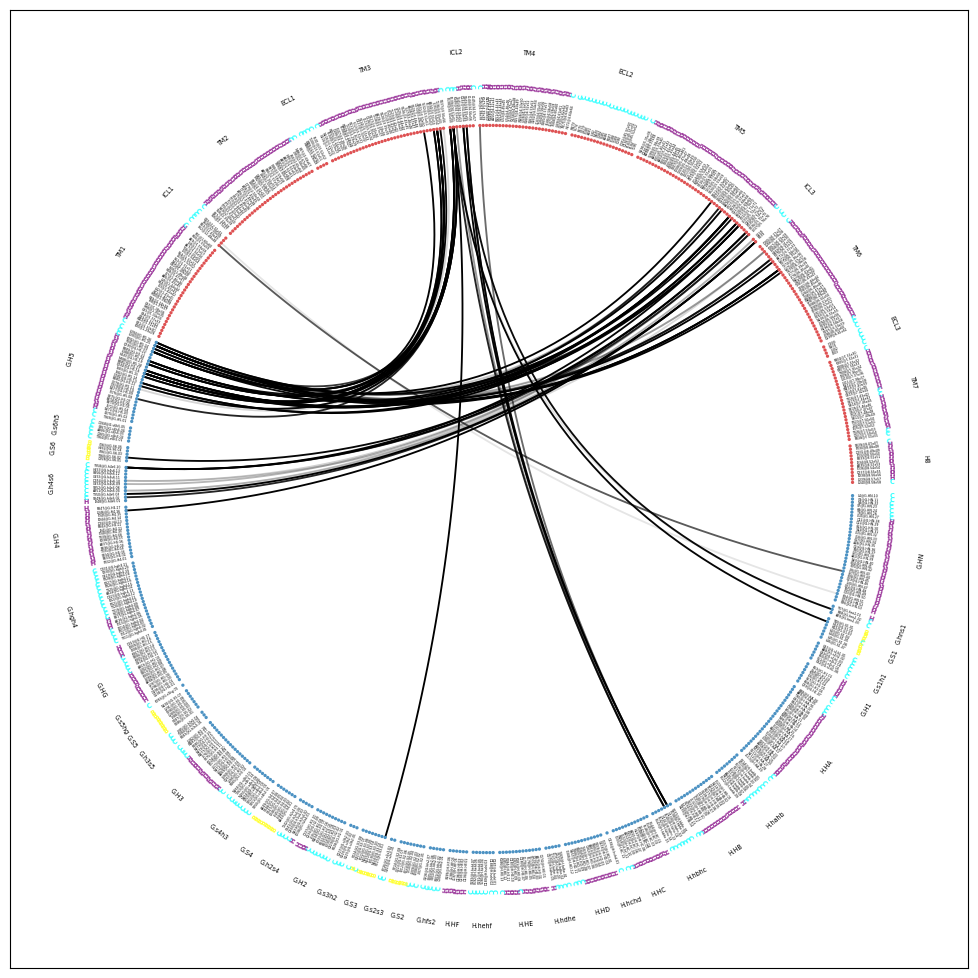
Additionally, we now have two other notebooks explicitly devoted to the representation of interfaces:
[15]:
mdciao.cli.interface(traj,
                     interface_selection_1=[0],
                     interface_selection_2=[3],
                     GPCR_UniProt=GPCR,
                     CGN_UniProt=CGN,
                     title="3SN6 beta2AR-Galpha interface",
                     accept_guess=True,
                     plot_timedep=False,
                     ctc_control=1.0,
                     no_disk=True)
Will compute contact frequencies for trajectories:
<mdtraj.Trajectory with 280 frames, 8384 atoms, 1044 residues, and unitcells>
 with a stride of 1 frames
Using method 'lig_resSeq+' these fragments were found
fragment 0 with    354 AAs     LEU4 (   0) -   LEU394 (353 ) (0) resSeq jumps
fragment 1 with    340 AAs     GLN1 ( 354) -   ASN340 (693 ) (1)
fragment 2 with     66 AAs     ALA2 ( 694) -    PHE67 (759 ) (2)
fragment 3 with    283 AAs    GLU30 ( 760) -   LEU340 (1042) (3) resSeq jumps
fragment 4 with      1 AAs   P0G395 (1043) -   P0G395 (1043) (4)
The GPCR-labels align best with fragments: [3] (first-last: GLU30-LEU340).

Mapping the GPCR fragments onto your topology:
 TM1  with     32 AAs    GLU30@1.29x29   ( 760) -    PHE61@1.60x60   (791 ) (TM1)
 ICL1 with      4 AAs    GLU62@12.48x48  ( 792) -    GLN65@12.51x51  (795 ) (ICL1)
 TM2  with     32 AAs    THR66@2.37x37   ( 796) -    LYS97@2.68x67   (827 ) (TM2)
 ECL1 with      4 AAs    MET98@23.49x49  ( 828) -   PHE101@23.52x52  (831 ) (ECL1)
 TM3  with     36 AAs   GLY102@3.21x21   ( 832) -   SER137@3.56x56   (867 ) (TM3)
 ICL2 with      8 AAs   PRO138@34.50x50  ( 868) -   LEU145@34.57x57  (875 ) (ICL2)
 TM4  with     27 AAs   THR146@4.38x38   ( 876) -   HIS172@4.64x64   (902 ) (TM4)
 ECL2 with     20 AAs   TRP173           ( 903) -   THR195           (922 ) (ECL2) resSeq jumps
 TM5  with     42 AAs   ASN196@5.35x36   ( 923) -   GLU237@5.76x76   (964 ) (TM5)
 ICL3 with      2 AAs   GLY238           ( 965) -   ARG239           (966 ) (ICL3)
 TM6  with     35 AAs   CYS265@6.27x27   ( 967) -   GLN299@6.61x61   (1001) (TM6)
 ECL3 with      4 AAs   ASP300           (1002) -   ILE303           (1005) (ECL3)
 TM7  with     25 AAs   ARG304@7.31x30   (1006) -   ARG328@7.55x55   (1030) (TM7)
 H8   with     12 AAs   SER329@8.47x47   (1031) -   LEU340@8.58x58   (1042) (H8)
The CGN-labels align best with fragments: [0] (first-last: LEU4-LEU394).

Mapping the CGN fragments onto your topology:
 G.HN   with     33 AAs     LEU4@G.HN.10   (   0) -    VAL36@G.HN.53   (32  ) (G.HN)
 G.hns1 with      3 AAs    TYR37@G.hns1.01 (  33) -    ALA39@G.hns1.03 (35  ) (G.hns1)
 G.S1   with      7 AAs    THR40@G.S1.01   (  36) -    LEU46@G.S1.07   (42  ) (G.S1)
 G.s1h1 with      6 AAs    GLY47@G.s1h1.01 (  43) -    GLY52@G.s1h1.06 (48  ) (G.s1h1)
 G.H1   with      7 AAs    LYS53@G.H1.01   (  49) -    GLN59@G.H1.07   (55  ) (G.H1)
 H.HA   with     26 AAs    LYS88@H.HA.04   (  56) -   LEU113@H.HA.29   (81  ) (H.HA)
 H.hahb with      9 AAs   VAL114@H.hahb.01 (  82) -   PRO122@H.hahb.09 (90  ) (H.hahb)
 H.HB   with     14 AAs   GLU123@H.HB.01   (  91) -   ASN136@H.HB.14   (104 ) (H.HB)
 H.hbhc with      7 AAs   VAL137@H.hbhc.01 ( 105) -   PRO143@H.hbhc.15 (111 ) (H.hbhc)
 H.HC   with     12 AAs   PRO144@H.HC.01   ( 112) -   GLU155@H.HC.12   (123 ) (H.HC)
 H.hchd with      1 AAs   ASP156@H.hchd.01 ( 124) -   ASP156@H.hchd.01 (124 ) (H.hchd)
 H.HD   with     12 AAs   GLU157@H.HD.01   ( 125) -   GLU168@H.HD.12   (136 ) (H.HD)
 H.hdhe with      5 AAs   TYR169@H.hdhe.01 ( 137) -   ASP173@H.hdhe.05 (141 ) (H.hdhe)
 H.HE   with     13 AAs   CYS174@H.HE.01   ( 142) -   LYS186@H.HE.13   (154 ) (H.HE)
 H.hehf with      7 AAs   GLN187@H.hehf.01 ( 155) -   SER193@H.hehf.07 (161 ) (H.hehf)
 H.HF   with      6 AAs   ASP194@H.HF.01   ( 162) -   ARG199@H.HF.06   (167 ) (H.HF)
 G.hfs2 with      5 AAs   CYS200@G.hfs2.01 ( 168) -   GLY206@G.hfs2.07 (172 ) (G.hfs2) resSeq jumps
 G.S2   with      8 AAs   ILE207@G.S2.01   ( 173) -   VAL214@G.S2.08   (180 ) (G.S2)
 G.s2s3 with      2 AAs   ASP215@G.s2s3.01 ( 181) -   LYS216@G.s2s3.02 (182 ) (G.s2s3)
 G.S3   with      8 AAs   VAL217@G.S3.01   ( 183) -   VAL224@G.S3.08   (190 ) (G.S3)
 G.s3h2 with      3 AAs   GLY225@G.s3h2.01 ( 191) -   GLN227@G.s3h2.03 (193 ) (G.s3h2)
 G.H2   with     10 AAs   ARG228@G.H2.01   ( 194) -   CYS237@G.H2.10   (203 ) (G.H2)
 G.h2s4 with      5 AAs   PHE238@G.h2s4.01 ( 204) -   THR242@G.h2s4.05 (208 ) (G.h2s4)
 G.S4   with      7 AAs   ALA243@G.S4.01   ( 209) -   ALA249@G.S4.07   (215 ) (G.S4)
 G.s4h3 with      8 AAs   SER250@G.s4h3.01 ( 216) -   ASN264@G.s4h3.15 (223 ) (G.s4h3) resSeq jumps
 G.H3   with     18 AAs   ARG265@G.H3.01   ( 224) -   LEU282@G.H3.18   (241 ) (G.H3)
 G.h3s5 with      3 AAs   ARG283@G.h3s5.01 ( 242) -   ILE285@G.h3s5.03 (244 ) (G.h3s5)
 G.S5   with      7 AAs   SER286@G.S5.01   ( 245) -   ASN292@G.S5.07   (251 ) (G.S5)
 G.s5hg with      1 AAs   LYS293@G.s5hg.01 ( 252) -   LYS293@G.s5hg.01 (252 ) (G.s5hg)
 G.HG   with     17 AAs   GLN294@G.HG.01   ( 253) -   ASP310@G.HG.17   (269 ) (G.HG)
 G.hgh4 with     21 AAs   TYR311@G.hgh4.01 ( 270) -   ASP331@G.hgh4.21 (290 ) (G.hgh4)
 G.H4   with     16 AAs   PRO332@G.H4.01   ( 291) -   ARG347@G.H4.17   (306 ) (G.H4)
 G.h4s6 with     11 AAs   ILE348@G.h4s6.01 ( 307) -   TYR358@G.h4s6.20 (317 ) (G.h4s6)
 G.S6   with      5 AAs   CYS359@G.S6.01   ( 318) -   PHE363@G.S6.05   (322 ) (G.S6)
 G.s6h5 with      5 AAs   THR364@G.s6h5.01 ( 323) -   ASP368@G.s6h5.05 (327 ) (G.s6h5)
 G.H5   with     26 AAs   THR369@G.H5.01   ( 328) -   LEU394@G.H5.26   (353 ) (G.H5)
Select group 1: 0
Select group 2: 3

Will look for contacts in the interface between fragments
0
and
3.

Performing a first pass on the 100182 group_1-group_2 residue pairs to compute lower bounds on residue-residue distances via residue-COM distances.
Reduced to only 912 (from 100182) residue pairs for the computation of actual residue-residue distances:
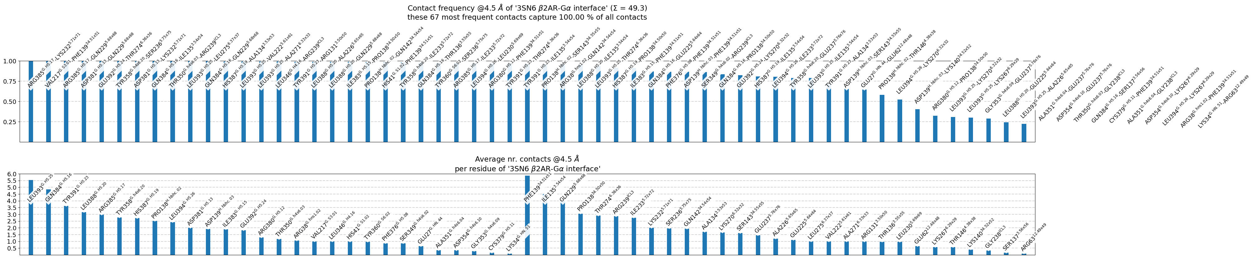
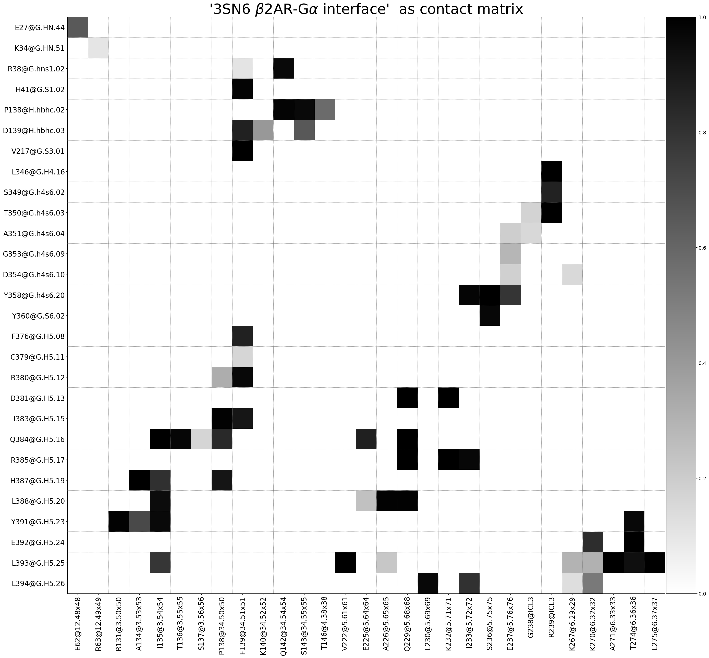
The following 67 contacts capture 49.26 (~98%) of the total frequency 50.28 (over 107 contacts with nonzero frequency at 4.50 Angstrom).
As orientation value, the first 50 ctcs already capture 90.0% of 50.28.
The 50-th contact has a frequency of 0.52.

    freq              label               residues  fragments   sum
1   1.00  R385@G.H5.17   - K232@5.71x71   344 - 959    0 - 3    1.00
2   1.00  V217@G.S3.01   - F139@34.51x51  183 - 869    0 - 3    2.00
3   1.00  R385@G.H5.17   - Q229@5.68x68   344 - 956    0 - 3    3.00
4   1.00  D381@G.H5.13   - Q229@5.68x68   340 - 956    0 - 3    4.00
5   1.00  E392@G.H5.24   - T274@6.36x36   351 - 976    0 - 3    5.00
6   1.00  Y358@G.h4s6.20 - S236@5.75x75   317 - 963    0 - 3    6.00
7   1.00  D381@G.H5.13   - K232@5.71x71   340 - 959    0 - 3    7.00
8   1.00  Q384@G.H5.16   - I135@3.54x54   343 - 865    0 - 3    8.00
9   1.00  T350@G.h4s6.03 - R239@ICL3      309 - 966    0 - 3    9.00
10  1.00  L393@G.H5.25   - L275@6.37x37   352 - 977    0 - 3    9.99
11  1.00  Q384@G.H5.16   - Q229@5.68x68   343 - 956    0 - 3   10.99
12  0.99  H387@G.H5.19   - A134@3.53x53   346 - 864    0 - 3   11.98
13  0.99  L393@G.H5.25   - V222@5.61x61   352 - 949    0 - 3   12.98
14  0.99  L393@G.H5.25   - A271@6.33x33   352 - 973    0 - 3   13.97
15  0.99  L346@G.H4.16   - R239@ICL3      305 - 966    0 - 3   14.96
16  0.99  Y391@G.H5.23   - R131@3.50x50   350 - 861    0 - 3   15.95
17  0.99  L388@G.H5.20   - A226@5.65x65   347 - 953    0 - 3   16.93
18  0.99  L388@G.H5.20   - Q229@5.68x68   347 - 956    0 - 3   17.92
19  0.99  I383@G.H5.15   - P138@34.50x50  342 - 868    0 - 3   18.90
20  0.98  P138@H.hbhc.02 - Q142@34.54x54  106 - 872    0 - 3   19.89
21  0.98  H41@G.S1.02    - F139@34.51x51   37 - 869    0 - 3   20.87
22  0.98  Y358@G.h4s6.20 - I233@5.72x72   317 - 960    0 - 3   21.85
23  0.98  Q384@G.H5.16   - T136@3.55x55   343 - 866    0 - 3   22.82
24  0.97  Y360@G.S6.02   - S236@5.75x75   319 - 963    0 - 3   23.79
25  0.97  R385@G.H5.17   - I233@5.72x72   344 - 960    0 - 3   24.76
26  0.97  L394@G.H5.26   - L230@5.69x69   353 - 957    0 - 3   25.73
27  0.97  R380@G.H5.12   - F139@34.51x51  339 - 869    0 - 3   26.70
28  0.96  Y391@G.H5.23   - T274@6.36x36   350 - 976    0 - 3   27.66
29  0.96  Y391@G.H5.23   - I135@3.54x54   350 - 865    0 - 3   28.63
30  0.96  P138@H.hbhc.02 - S143@34.55x55  106 - 873    0 - 3   29.58
31  0.96  R38@G.hns1.02  - Q142@34.54x54   34 - 872    0 - 3   30.54
32  0.95  L388@G.H5.20   - I135@3.54x54   347 - 865    0 - 3   31.49
33  0.94  L393@G.H5.25   - T274@6.36x36   352 - 976    0 - 3   32.43
34  0.91  H387@G.H5.19   - P138@34.50x50  346 - 868    0 - 3   33.34
35  0.91  I383@G.H5.15   - F139@34.51x51  342 - 869    0 - 3   34.25
36  0.87  Q384@G.H5.16   - E225@5.64x64   343 - 952    0 - 3   35.12
37  0.86  F376@G.H5.08   - F139@34.51x51  335 - 869    0 - 3   35.99
38  0.86  D139@H.hbhc.03 - F139@34.51x51  107 - 869    0 - 3   36.85
39  0.86  S349@G.h4s6.02 - R239@ICL3      308 - 966    0 - 3   37.71
40  0.83  Q384@G.H5.16   - P138@34.50x50  343 - 868    0 - 3   38.54
41  0.82  E392@G.H5.24   - K270@6.32x32   351 - 972    0 - 3   39.36
42  0.81  H387@G.H5.19   - I135@3.54x54   346 - 865    0 - 3   40.17
43  0.80  L394@G.H5.26   - I233@5.72x72   353 - 960    0 - 3   40.97
44  0.79  Y358@G.h4s6.20 - E237@5.76x76   317 - 964    0 - 3   41.76
45  0.79  L393@G.H5.25   - I135@3.54x54   352 - 865    0 - 3   42.55
46  0.71  Y391@G.H5.23   - A134@3.53x53   350 - 864    0 - 3   43.26
47  0.65  D139@H.hbhc.03 - S143@34.55x55  107 - 873    0 - 3   43.91
48  0.65  E27@G.HN.44    - E62@12.48x48    23 - 792    0 - 3   44.56
49  0.58  P138@H.hbhc.02 - T146@4.38x38   106 - 876    0 - 3   45.14
50  0.52  L394@G.H5.26   - K270@6.32x32   353 - 972    0 - 3   45.66
51  0.40  D139@H.hbhc.03 - K140@34.52x52  107 - 870    0 - 3   46.06
52  0.32  R380@G.H5.12   - P138@34.50x50  339 - 868    0 - 3   46.39
53  0.31  L393@G.H5.25   - K270@6.32x32   352 - 972    0 - 3   46.69
54  0.30  L393@G.H5.25   - K267@6.29x29   352 - 969    0 - 3   46.99
55  0.29  G353@G.h4s6.09 - E237@5.76x76   312 - 964    0 - 3   47.28
56  0.24  L388@G.H5.20   - E225@5.64x64   347 - 952    0 - 3   47.52
57  0.22  L393@G.H5.25   - A226@5.65x65   352 - 953    0 - 3   47.74
58  0.19  A351@G.h4s6.04 - E237@5.76x76   310 - 964    0 - 3   47.94
59  0.19  D354@G.h4s6.10 - E237@5.76x76   313 - 964    0 - 3   48.12
60  0.17  T350@G.h4s6.03 - G238@ICL3      309 - 965    0 - 3   48.29
61  0.16  Q384@G.H5.16   - S137@3.56x56   343 - 867    0 - 3   48.46
62  0.16  C379@G.H5.11   - F139@34.51x51  338 - 869    0 - 3   48.62
63  0.15  A351@G.h4s6.04 - G238@ICL3      310 - 965    0 - 3   48.77
64  0.15  D354@G.h4s6.10 - K267@6.29x29   313 - 969    0 - 3   48.92
65  0.13  L394@G.H5.26   - K267@6.29x29   353 - 969    0 - 3   49.05
66  0.11  R38@G.hns1.02  - F139@34.51x51   34 - 869    0 - 3   49.16
67  0.10  K34@G.HN.51    - R63@12.49x49    30 - 793    0 - 3   49.26

             label  freq
1     L393@G.H5.25  5.54
2     Q384@G.H5.16  4.84
3     Y391@G.H5.23  3.62
4     L388@G.H5.20  3.16
5     R385@G.H5.17  2.97
6   Y358@G.h4s6.20  2.77
7     H387@G.H5.19  2.71
8   P138@H.hbhc.02  2.52
9     L394@G.H5.26  2.42
10    D381@G.H5.13  2.00
11  D139@H.hbhc.03  1.92
12    I383@G.H5.15  1.90
13    E392@G.H5.24  1.82
14    R380@G.H5.12  1.29
15  T350@G.h4s6.03  1.17
16   R38@G.hns1.02  1.06
17    V217@G.S3.01  1.00
18    L346@G.H4.16  0.99
19     H41@G.S1.02  0.98
20    Y360@G.S6.02  0.97
21    F376@G.H5.08  0.86
22  S349@G.h4s6.02  0.86
23     E27@G.HN.44  0.65
24  A351@G.h4s6.04  0.35
25  D354@G.h4s6.10  0.34
26  G353@G.h4s6.09  0.29
27    C379@G.H5.11  0.16
28     K34@G.HN.51  0.10

            label  freq
1   F139@34.51x51  5.86
2    I135@3.54x54  4.50
3    Q229@5.68x68  3.98
4   P138@34.50x50  3.05
5    T274@6.36x36  2.90
6       R239@ICL3  2.85
7    I233@5.72x72  2.75
8    K232@5.71x71  2.00
9    S236@5.75x75  1.97
10  Q142@34.54x54  1.94
11   A134@3.53x53  1.70
12   K270@6.32x32  1.65
13  S143@34.55x55  1.61
14   E237@5.76x76  1.45
15   A226@5.65x65  1.21
16   E225@5.64x64  1.11
17   L275@6.37x37  1.00
18   V222@5.61x61  0.99
19   A271@6.33x33  0.99
20   R131@3.50x50  0.99
21   T136@3.55x55  0.98
22   L230@5.69x69  0.97
23   E62@12.48x48  0.65
24   K267@6.29x29  0.58
25   T146@4.38x38  0.58
26  K140@34.52x52  0.40
27      G238@ICL3  0.32
28   S137@3.56x56  0.16
29   R63@12.49x49  0.10

Drawing this many dots (637 residues + 52 padding spaces) in a panel 10.0 inches wide/high
forces too small dotsizes and fontsizes. If crowding effects occur, either reduce the
number of residues or increase the panel size
[15]:
<mdciao.contacts.contacts.ContactGroup at 0x79d262716350>
Sites
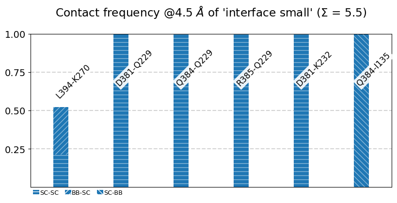
Now we use a different approach. Instead of letting mdciao discover contacts automatically, we list them beforehand as site dictionaries, and feed this dictionaries to directly to the method cli.sites. The CLI command we’re replicating is:
mdc_sites.py top.pdb traj.xtc --site tip.json -at -nf -sa #sa: short AA-names
However, in the API-spirit, we’re not even using a file on disk to define the site, but create it on the fly as a Python dictionary:
[16]:
my_site = {
    "name":"interface small",
    "pairs": {"AAresSeq": [
        "L394-K270",
        "D381-Q229",
        "Q384-Q229",
        "R385-Q229",
        "D381-K232",
        "Q384-I135"
        ]}}
[17]:
sites = mdciao.cli.sites(my_site,
                         traj,
                         no_disk=True,
                         plot_atomtypes=True,
                         fragments=None,
                         short_AA_names=True)
Will compute the sites
 site dict with name 'interface small'
in the trajectories:
<mdtraj.Trajectory with 280 frames, 8384 atoms, 1044 residues, and unitcells>
 with a stride of 1 frames.

Using method 'None' these fragments were found
fragment 0 with   1044 AAs     LEU4 (   0) -   P0G395 (1043) (0) resSeq jumps
These are the residues that could be found:
   residue      residx    fragment      resSeq
    ASP381         340           0         381
    GLN384         343           0         384
    ARG385         344           0         385
    LEU394         353           0         394
    ILE135         865           0         135
    GLN229         956           0         229
    LYS232         959           0         232
    LYS270         972           0         270
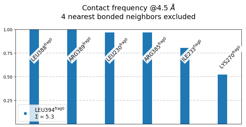
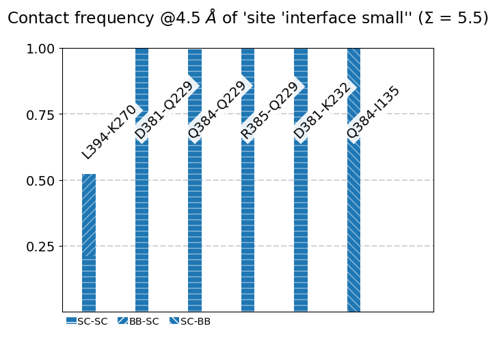
Site 'interface small':
   freq        label   residues fragments   sum
0  0.52  L394 - K270  353 - 972     0 - 0  0.52
1  1.00  D381 - Q229  340 - 956     0 - 0  1.52
2  1.00  Q384 - Q229  343 - 956     0 - 0  2.52
3  1.00  R385 - Q229  344 - 956     0 - 0  3.52
4  1.00  D381 - K232  340 - 959     0 - 0  4.52
5  1.00  Q384 - I135  343 - 865     0 - 0  5.52
The return value sites is a dictionary keyed with the site names (interface small in this case) and valued with mdciao's ContactGroup-objects.
[18]:
sites
[18]:
{'interface small': <mdciao.contacts.contacts.ContactGroup at 0x79d2619080d0>}
Contact Groups
The ContactGroup class is at the center of mdciao and offers extensive of manipulation through it’s methods. A helpful analogy would be that, what the Trajectory is to mdtraj, the
ContactGroup is to mdciao. Both classes:
store a lot of organized information for further use
have attributes and methods that can be used standalone
can themselves be the input for other methods (of
mdtrajandmdciao, respectively).are rarely created from scratch, but rather generated by the module itself.
The best way to learn about the ContactGroup is to inspect it with the autocomplete feature if IPython and check the informative names of the attributes and methods.
If you’re in a hurry, mdciao offers a quick way to generate a ContactGroup to play around with and investigate it’s methods and attributes:
[19]:
from mdciao import examples
CG = examples.ContactGroupL394()
CG
[19]:
<mdciao.contacts.contacts.ContactGroup at 0x79d2a8de8c10>
However, instead of using CG now, we go back to object sites that resulted from using cli.sites above. The returned sites-object is a dictionary keyed with site names (you can compute different sites simultaneously) and valued with ContactGroups. In our case (check above) we called it it interface small
[20]:
mysite = sites["interface small"]
Frequencies as Bars
We use the class’s method plot_freqs_as_bars to produce the now familiar neighborhood plots:
[21]:
mysite.plot_freqs_as_bars(4.5,
                          shorten_AAs=True,
                          defrag="@",
                          plot_atomtypes=True);
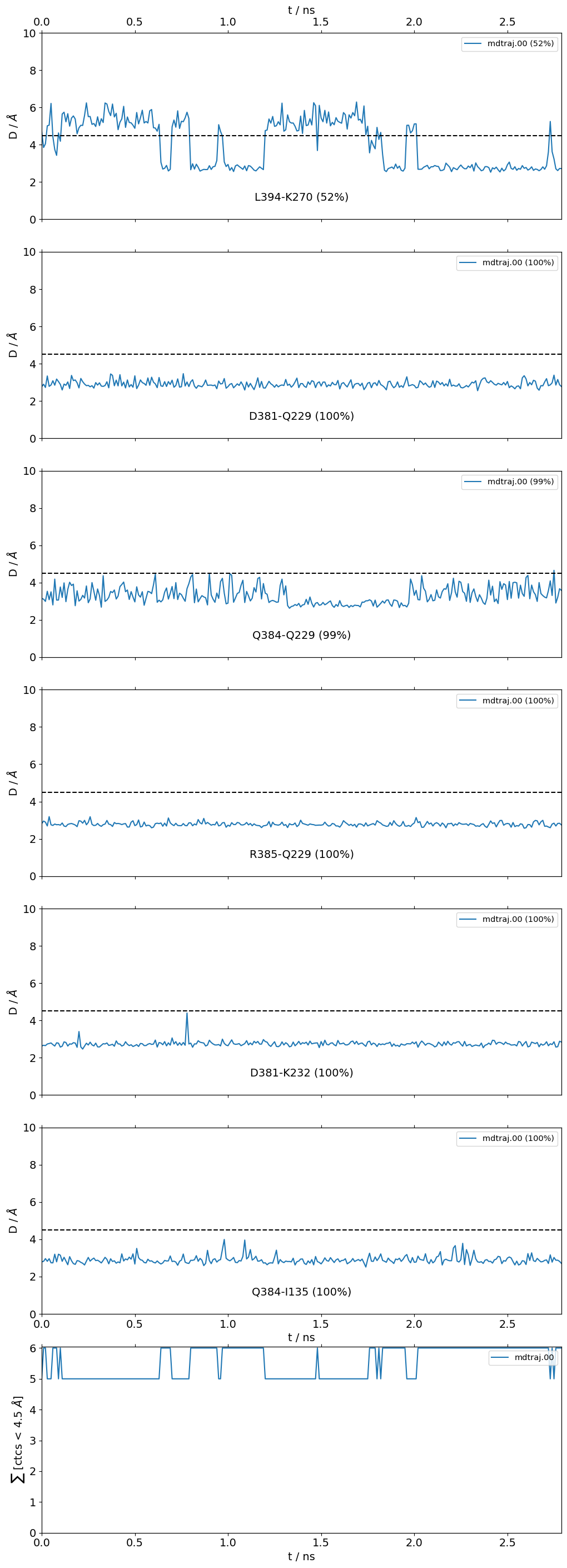
Frequencies as Distributions
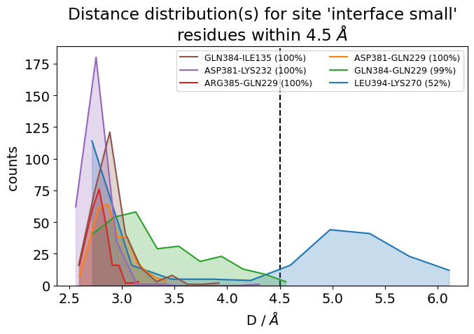
It is also very useful to inspect the residue-residue distances of any ContactGroup by looking at their overall distributions instead of their frequencies, since the hard cutoffs can sometimes hide part of the story:
[22]:
jax = mysite.plot_distance_distributions(defrag="@",
                                         ctc_cutoff_Ang=4.5
                                        )
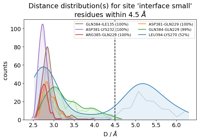
Please note that, because the example dataset is quite small (280 frames and 2.8 ns) and we are simply histogramming (=counting), the curves aren’t very smooth. Histograms of real data will look better.
What we can do is use the smooth_bw keyword to smooth a bit the noisy histograms use a kernel-density estimation using Gaussian kernels. The smooth_bw parameter has a default bandwidth value of .5 Angstrom (which usually yields good results), but you can adjust it, e.g. here we’ve changed it to .25.
[23]:
jax = mysite.plot_distance_distributions(bins=20,
                                         defrag="@",
                                         ctc_cutoff_Ang=4.5,
                                         smooth_bw=.25
                                        )
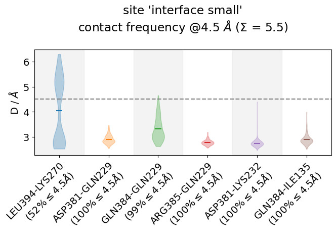
Frequencies as Violins
Other ways of looking at distance-data as distributions is to use violin plots, which uses a density estimator (check the bw_method-parameter here) to generate smooth densities and plot them vertically. This is somehow in-between the histogram plot and the
frequency-bar plot:
[24]:
jax = mysite.plot_violins(defrag="@",
                          ctc_cutoff_Ang=4.5,
                          color="tab10",
                         )
Comparisons Between Contact Groups
Finally, we replicate the CLI comand
mdc_compare.py 3SN6.X.ARG131@4.0_Ang.dat 3SN6.MD.ARG131@4.0_Ang.dat -k Xray,MD -t "3SN6 cutoff 4AA" -a R131
in API mode. This looks different because most of the inputs will now be Python objects in memory.
First, we create the Xray and the MD ContactGroups separately:
[25]:
R131_Xray = mdciao.cli.residue_neighborhoods("R131", xray3SN6,
                                             ctc_cutoff_Ang=4.5,
                                             no_disk=True,
                                             GPCR_UniProt=GPCR,
                                             figures=False,
                                             CGN_UniProt=CGN,
                                             accept_guess=True)
Will compute contact frequencies for (1 items):
<mdtraj.Trajectory with 1 frames, 10274 atoms, 1319 residues, and unitcells>
 with a stride of 1 frames
Using method 'lig_resSeq+' these fragments were found
fragment 0 with    349 AAs     THR9 (   0) -   LEU394 (348 ) (0) resSeq jumps
fragment 1 with    340 AAs     GLN1 ( 349) -   ASN340 (688 ) (1)
fragment 2 with     58 AAs     ASN5 ( 689) -    ARG62 (746 ) (2)
fragment 3 with    159 AAs  ASN1002 ( 747) -  ALA1160 (905 ) (3)
fragment 4 with    284 AAs    GLU30 ( 906) -   CYS341 (1189) (4) resSeq jumps
fragment 5 with    128 AAs     GLN1 (1190) -   SER128 (1317) (5)
fragment 6 with      1 AAs  P0G1601 (1318) -  P0G1601 (1318) (6)
The GPCR-labels align best with fragments: [4] (first-last: GLU30-CYS341).

Mapping the GPCR fragments onto your topology:
 TM1  with     32 AAs    GLU30@1.29x29   ( 906) -    PHE61@1.60x60   (937 ) (TM1)
 ICL1 with      4 AAs    GLU62@12.48x48  ( 938) -    GLN65@12.51x51  (941 ) (ICL1)
 TM2  with     32 AAs    THR66@2.37x37   ( 942) -    LYS97@2.68x67   (973 ) (TM2)
 ECL1 with      4 AAs    THR98@23.49x49  ( 974) -   PHE101@23.52x52  (977 ) (ECL1)
 TM3  with     36 AAs   GLY102@3.21x21   ( 978) -   SER137@3.56x56   (1013) (TM3)
 ICL2 with      8 AAs   PRO138@34.50x50  (1014) -   LEU145@34.57x57  (1021) (ICL2)
 TM4  with     27 AAs   THR146@4.38x38   (1022) -   HIS172@4.64x64   (1048) (TM4)
 ECL2 with     20 AAs   TRP173           (1049) -   THR195           (1068) (ECL2) resSeq jumps
 TM5  with     42 AAs   ASN196@5.35x36   (1069) -   GLU237@5.76x76   (1110) (TM5)
 ICL3 with      2 AAs   GLY238           (1111) -   ARG239           (1112) (ICL3)
 TM6  with     35 AAs   CYS265@6.27x27   (1113) -   GLN299@6.61x61   (1147) (TM6)
 ECL3 with      4 AAs   ASP300           (1148) -   ILE303           (1151) (ECL3)
 TM7  with     25 AAs   ARG304@7.31x30   (1152) -   ARG328@7.55x55   (1176) (TM7)
 H8   with     13 AAs   SER329@8.47x47   (1177) -   CYS341@8.59x59   (1189) (H8)
The CGN-labels align best with fragments: [0] (first-last: THR9-LEU394).

Mapping the CGN fragments onto your topology:
 G.HN   with     28 AAs     THR9@G.HN.26   (   0) -    VAL36@G.HN.53   (27  ) (G.HN)
 G.hns1 with      3 AAs    TYR37@G.hns1.01 (  28) -    ALA39@G.hns1.03 (30  ) (G.hns1)
 G.S1   with      7 AAs    THR40@G.S1.01   (  31) -    LEU46@G.S1.07   (37  ) (G.S1)
 G.s1h1 with      6 AAs    GLY47@G.s1h1.01 (  38) -    GLY52@G.s1h1.06 (43  ) (G.s1h1)
 G.H1   with      7 AAs    LYS53@G.H1.01   (  44) -    GLN59@G.H1.07   (50  ) (G.H1)
 H.HA   with     26 AAs    LYS88@H.HA.04   (  51) -   LEU113@H.HA.29   (76  ) (H.HA)
 H.hahb with      9 AAs   VAL114@H.hahb.01 (  77) -   PRO122@H.hahb.09 (85  ) (H.hahb)
 H.HB   with     14 AAs   GLU123@H.HB.01   (  86) -   ASN136@H.HB.14   (99  ) (H.HB)
 H.hbhc with      7 AAs   VAL137@H.hbhc.01 ( 100) -   PRO143@H.hbhc.15 (106 ) (H.hbhc)
 H.HC   with     12 AAs   PRO144@H.HC.01   ( 107) -   GLU155@H.HC.12   (118 ) (H.HC)
 H.hchd with      1 AAs   ASP156@H.hchd.01 ( 119) -   ASP156@H.hchd.01 (119 ) (H.hchd)
 H.HD   with     12 AAs   GLU157@H.HD.01   ( 120) -   GLU168@H.HD.12   (131 ) (H.HD)
 H.hdhe with      5 AAs   TYR169@H.hdhe.01 ( 132) -   ASP173@H.hdhe.05 (136 ) (H.hdhe)
 H.HE   with     13 AAs   CYS174@H.HE.01   ( 137) -   LYS186@H.HE.13   (149 ) (H.HE)
 H.hehf with      7 AAs   GLN187@H.hehf.01 ( 150) -   SER193@H.hehf.07 (156 ) (H.hehf)
 H.HF   with      6 AAs   ASP194@H.HF.01   ( 157) -   ARG199@H.HF.06   (162 ) (H.HF)
 G.hfs2 with      5 AAs   CYS200@G.hfs2.01 ( 163) -   GLY206@G.hfs2.07 (167 ) (G.hfs2) resSeq jumps
 G.S2   with      8 AAs   ILE207@G.S2.01   ( 168) -   VAL214@G.S2.08   (175 ) (G.S2)
 G.s2s3 with      2 AAs   ASP215@G.s2s3.01 ( 176) -   LYS216@G.s2s3.02 (177 ) (G.s2s3)
 G.S3   with      8 AAs   VAL217@G.S3.01   ( 178) -   VAL224@G.S3.08   (185 ) (G.S3)
 G.s3h2 with      3 AAs   GLY225@G.s3h2.01 ( 186) -   GLN227@G.s3h2.03 (188 ) (G.s3h2)
 G.H2   with     10 AAs   ARG228@G.H2.01   ( 189) -   CYS237@G.H2.10   (198 ) (G.H2)
 G.h2s4 with      5 AAs   PHE238@G.h2s4.01 ( 199) -   THR242@G.h2s4.05 (203 ) (G.h2s4)
 G.S4   with      7 AAs   ALA243@G.S4.01   ( 204) -   ALA249@G.S4.07   (210 ) (G.S4)
 G.s4h3 with      8 AAs   SER250@G.s4h3.01 ( 211) -   ASN264@G.s4h3.15 (218 ) (G.s4h3) resSeq jumps
 G.H3   with     18 AAs   ARG265@G.H3.01   ( 219) -   LEU282@G.H3.18   (236 ) (G.H3)
 G.h3s5 with      3 AAs   ARG283@G.h3s5.01 ( 237) -   ILE285@G.h3s5.03 (239 ) (G.h3s5)
 G.S5   with      7 AAs   SER286@G.S5.01   ( 240) -   ASN292@G.S5.07   (246 ) (G.S5)
 G.s5hg with      1 AAs   LYS293@G.s5hg.01 ( 247) -   LYS293@G.s5hg.01 (247 ) (G.s5hg)
 G.HG   with     17 AAs   GLN294@G.HG.01   ( 248) -   ASP310@G.HG.17   (264 ) (G.HG)
 G.hgh4 with     21 AAs   TYR311@G.hgh4.01 ( 265) -   ASP331@G.hgh4.21 (285 ) (G.hgh4)
 G.H4   with     16 AAs   PRO332@G.H4.01   ( 286) -   ARG347@G.H4.17   (301 ) (G.H4)
 G.h4s6 with     11 AAs   ILE348@G.h4s6.01 ( 302) -   TYR358@G.h4s6.20 (312 ) (G.h4s6)
 G.S6   with      5 AAs   CYS359@G.S6.01   ( 313) -   PHE363@G.S6.05   (317 ) (G.S6)
 G.s6h5 with      5 AAs   THR364@G.s6h5.01 ( 318) -   ASP368@G.s6h5.05 (322 ) (G.s6h5)
 G.H5   with     26 AAs   THR369@G.H5.01   ( 323) -   LEU394@G.H5.26   (348 ) (G.H5)

Will compute neighborhoods for the residues
R131
excluding 4 nearest neighbors

   residue      residx    fragment      resSeq        GPCR         CGN
    ARG131        1007           4         131     3.50x50        None

Performing a first pass on 1310 residue pairs to compute lower bounds on residue-residue distances via residue-COM distances:
Reduced to only 59 residue pairs for the computation of actual residue-residue distances:
R131@3.50x50:
The following 5 contacts capture 5.00 (~100%) of the total frequency 5.00 (over 5 contacts with nonzero frequency at 4.50 Angstrom).
As orientation value, the first 5 ctcs already capture 90.0% of 5.00.
The 5-th contact has a frequency of 1.00.
   freq            label               residues   fragments  sum
1   1.0  R131@3.50x50 - Y326@7.53x53  1007 - 1174    4 - 4   1.0
2   1.0  R131@3.50x50 - Y391@G.H5.23   1007 - 345    4 - 0   2.0
3   1.0  R131@3.50x50 - V222@5.61x61  1007 - 1095    4 - 4   3.0
4   1.0  R131@3.50x50 - Y219@5.58x58  1007 - 1092    4 - 4   4.0
5   1.0  R131@3.50x50 - I278@6.40x40  1007 - 1126    4 - 4   5.0
[26]:
R131_MD = mdciao.cli.residue_neighborhoods("R131",traj,
                                           ctc_cutoff_Ang=4.5,
                                           no_disk=True,
                                           GPCR_UniProt=GPCR,
                                           figures=False,
                                           CGN_UniProt=CGN,
                                           accept_guess=True)
Will compute contact frequencies for (1 items):
<mdtraj.Trajectory with 280 frames, 8384 atoms, 1044 residues, and unitcells>
 with a stride of 1 frames
Using method 'lig_resSeq+' these fragments were found
fragment 0 with    354 AAs     LEU4 (   0) -   LEU394 (353 ) (0) resSeq jumps
fragment 1 with    340 AAs     GLN1 ( 354) -   ASN340 (693 ) (1)
fragment 2 with     66 AAs     ALA2 ( 694) -    PHE67 (759 ) (2)
fragment 3 with    283 AAs    GLU30 ( 760) -   LEU340 (1042) (3) resSeq jumps
fragment 4 with      1 AAs   P0G395 (1043) -   P0G395 (1043) (4)
The GPCR-labels align best with fragments: [3] (first-last: GLU30-LEU340).

Mapping the GPCR fragments onto your topology:
 TM1  with     32 AAs    GLU30@1.29x29   ( 760) -    PHE61@1.60x60   (791 ) (TM1)
 ICL1 with      4 AAs    GLU62@12.48x48  ( 792) -    GLN65@12.51x51  (795 ) (ICL1)
 TM2  with     32 AAs    THR66@2.37x37   ( 796) -    LYS97@2.68x67   (827 ) (TM2)
 ECL1 with      4 AAs    MET98@23.49x49  ( 828) -   PHE101@23.52x52  (831 ) (ECL1)
 TM3  with     36 AAs   GLY102@3.21x21   ( 832) -   SER137@3.56x56   (867 ) (TM3)
 ICL2 with      8 AAs   PRO138@34.50x50  ( 868) -   LEU145@34.57x57  (875 ) (ICL2)
 TM4  with     27 AAs   THR146@4.38x38   ( 876) -   HIS172@4.64x64   (902 ) (TM4)
 ECL2 with     20 AAs   TRP173           ( 903) -   THR195           (922 ) (ECL2) resSeq jumps
 TM5  with     42 AAs   ASN196@5.35x36   ( 923) -   GLU237@5.76x76   (964 ) (TM5)
 ICL3 with      2 AAs   GLY238           ( 965) -   ARG239           (966 ) (ICL3)
 TM6  with     35 AAs   CYS265@6.27x27   ( 967) -   GLN299@6.61x61   (1001) (TM6)
 ECL3 with      4 AAs   ASP300           (1002) -   ILE303           (1005) (ECL3)
 TM7  with     25 AAs   ARG304@7.31x30   (1006) -   ARG328@7.55x55   (1030) (TM7)
 H8   with     12 AAs   SER329@8.47x47   (1031) -   LEU340@8.58x58   (1042) (H8)
The CGN-labels align best with fragments: [0] (first-last: LEU4-LEU394).

Mapping the CGN fragments onto your topology:
 G.HN   with     33 AAs     LEU4@G.HN.10   (   0) -    VAL36@G.HN.53   (32  ) (G.HN)
 G.hns1 with      3 AAs    TYR37@G.hns1.01 (  33) -    ALA39@G.hns1.03 (35  ) (G.hns1)
 G.S1   with      7 AAs    THR40@G.S1.01   (  36) -    LEU46@G.S1.07   (42  ) (G.S1)
 G.s1h1 with      6 AAs    GLY47@G.s1h1.01 (  43) -    GLY52@G.s1h1.06 (48  ) (G.s1h1)
 G.H1   with      7 AAs    LYS53@G.H1.01   (  49) -    GLN59@G.H1.07   (55  ) (G.H1)
 H.HA   with     26 AAs    LYS88@H.HA.04   (  56) -   LEU113@H.HA.29   (81  ) (H.HA)
 H.hahb with      9 AAs   VAL114@H.hahb.01 (  82) -   PRO122@H.hahb.09 (90  ) (H.hahb)
 H.HB   with     14 AAs   GLU123@H.HB.01   (  91) -   ASN136@H.HB.14   (104 ) (H.HB)
 H.hbhc with      7 AAs   VAL137@H.hbhc.01 ( 105) -   PRO143@H.hbhc.15 (111 ) (H.hbhc)
 H.HC   with     12 AAs   PRO144@H.HC.01   ( 112) -   GLU155@H.HC.12   (123 ) (H.HC)
 H.hchd with      1 AAs   ASP156@H.hchd.01 ( 124) -   ASP156@H.hchd.01 (124 ) (H.hchd)
 H.HD   with     12 AAs   GLU157@H.HD.01   ( 125) -   GLU168@H.HD.12   (136 ) (H.HD)
 H.hdhe with      5 AAs   TYR169@H.hdhe.01 ( 137) -   ASP173@H.hdhe.05 (141 ) (H.hdhe)
 H.HE   with     13 AAs   CYS174@H.HE.01   ( 142) -   LYS186@H.HE.13   (154 ) (H.HE)
 H.hehf with      7 AAs   GLN187@H.hehf.01 ( 155) -   SER193@H.hehf.07 (161 ) (H.hehf)
 H.HF   with      6 AAs   ASP194@H.HF.01   ( 162) -   ARG199@H.HF.06   (167 ) (H.HF)
 G.hfs2 with      5 AAs   CYS200@G.hfs2.01 ( 168) -   GLY206@G.hfs2.07 (172 ) (G.hfs2) resSeq jumps
 G.S2   with      8 AAs   ILE207@G.S2.01   ( 173) -   VAL214@G.S2.08   (180 ) (G.S2)
 G.s2s3 with      2 AAs   ASP215@G.s2s3.01 ( 181) -   LYS216@G.s2s3.02 (182 ) (G.s2s3)
 G.S3   with      8 AAs   VAL217@G.S3.01   ( 183) -   VAL224@G.S3.08   (190 ) (G.S3)
 G.s3h2 with      3 AAs   GLY225@G.s3h2.01 ( 191) -   GLN227@G.s3h2.03 (193 ) (G.s3h2)
 G.H2   with     10 AAs   ARG228@G.H2.01   ( 194) -   CYS237@G.H2.10   (203 ) (G.H2)
 G.h2s4 with      5 AAs   PHE238@G.h2s4.01 ( 204) -   THR242@G.h2s4.05 (208 ) (G.h2s4)
 G.S4   with      7 AAs   ALA243@G.S4.01   ( 209) -   ALA249@G.S4.07   (215 ) (G.S4)
 G.s4h3 with      8 AAs   SER250@G.s4h3.01 ( 216) -   ASN264@G.s4h3.15 (223 ) (G.s4h3) resSeq jumps
 G.H3   with     18 AAs   ARG265@G.H3.01   ( 224) -   LEU282@G.H3.18   (241 ) (G.H3)
 G.h3s5 with      3 AAs   ARG283@G.h3s5.01 ( 242) -   ILE285@G.h3s5.03 (244 ) (G.h3s5)
 G.S5   with      7 AAs   SER286@G.S5.01   ( 245) -   ASN292@G.S5.07   (251 ) (G.S5)
 G.s5hg with      1 AAs   LYS293@G.s5hg.01 ( 252) -   LYS293@G.s5hg.01 (252 ) (G.s5hg)
 G.HG   with     17 AAs   GLN294@G.HG.01   ( 253) -   ASP310@G.HG.17   (269 ) (G.HG)
 G.hgh4 with     21 AAs   TYR311@G.hgh4.01 ( 270) -   ASP331@G.hgh4.21 (290 ) (G.hgh4)
 G.H4   with     16 AAs   PRO332@G.H4.01   ( 291) -   ARG347@G.H4.17   (306 ) (G.H4)
 G.h4s6 with     11 AAs   ILE348@G.h4s6.01 ( 307) -   TYR358@G.h4s6.20 (317 ) (G.h4s6)
 G.S6   with      5 AAs   CYS359@G.S6.01   ( 318) -   PHE363@G.S6.05   (322 ) (G.S6)
 G.s6h5 with      5 AAs   THR364@G.s6h5.01 ( 323) -   ASP368@G.s6h5.05 (327 ) (G.s6h5)
 G.H5   with     26 AAs   THR369@G.H5.01   ( 328) -   LEU394@G.H5.26   (353 ) (G.H5)

Will compute neighborhoods for the residues
R131
excluding 4 nearest neighbors

   residue      residx    fragment      resSeq        GPCR         CGN
    ARG131         861           3         131     3.50x50        None

Performing a first pass on 1035 residue pairs to compute lower bounds on residue-residue distances via residue-COM distances:
Reduced to only 75 residue pairs for the computation of actual residue-residue distances:
R131@3.50x50:
The following 6 contacts capture 3.15 (~99%) of the total frequency 3.17 (over 7 contacts with nonzero frequency at 4.50 Angstrom).
As orientation value, the first 4 ctcs already capture 90.0% of 3.17.
The 4-th contact has a frequency of 0.39.
   freq            label               residues  fragments   sum
1  0.99  R131@3.50x50 - Y391@G.H5.23   861 - 350    3 - 0   0.99
2  0.94  R131@3.50x50 - Y326@7.53x53  861 - 1028    3 - 3   1.92
3  0.76  R131@3.50x50 - Y219@5.58x58   861 - 946    3 - 3   2.69
4  0.39  R131@3.50x50 - I278@6.40x40   861 - 980    3 - 3   3.07
5  0.05  R131@3.50x50 - I325@7.52x52  861 - 1027    3 - 3   3.12
6  0.02  R131@3.50x50 - I72@2.43x43    861 - 802    3 - 3   3.15
Please note that, because the molecular topologies differ, the residue R131 is has different indices in each topology, namely 1007 in the X-ray crystal, 861 in the MD simulation:
[27]:
R131_Xray, R131_MD
[27]:
({1007: <mdciao.contacts.contacts.ContactGroup at 0x79d2a8805310>},
 {861: <mdciao.contacts.contacts.ContactGroup at 0x79d2a8c17050>})
That will frequently be the case when comparing different proteins of the same family, or topologies where not all sub-units have been modelled, termini have been differently cropped or anything that produces a shift in these indices.
mdciao understands R131 automatically and doesn’t ask more questions, as long as there’s an obvious R131 candidate. Otherwise the user will be prompted for disambiguation.
In this case, now we create a dictionary of ContactGroups that represent the R131 in both topologies:
[28]:
R131 = {
    "Xray": R131_Xray[1007],
    "MD"  : R131_MD[861]
}
#np.save("R131.npz",R131)
Now we can just pass this dictionary to cli.compare to see their contact frequencies. This method is pretty flexible on inputs and outputs, check the documentation to learn more:
[29]:
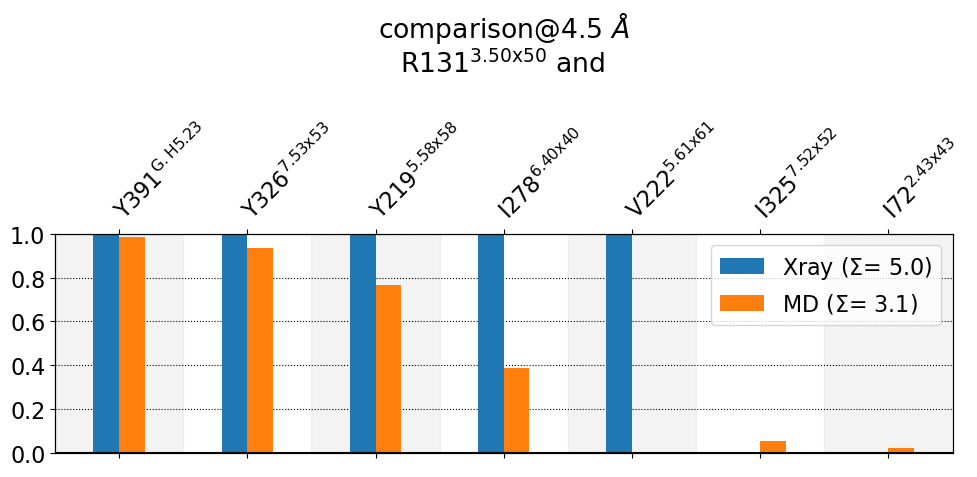
mdciao.cli.compare(R131, ctc_cutoff_Ang=4.5, defrag=None, anchor="R131");
These interactions are not shared:
I325@7.52x52, I72@2.43x43, V222@5.61x61
Their cumulative ctc freq is 1.07.
Created files
freq_comparison.pdf
freq_comparison.xlsx