Covid-19 Spike Protein Example 2: RBD-ACE Interface

In this notebook, we use mdciao to analyse publicly available MD data of the Covid-19 Spike Protein, curated in the impressive **COVID-19 Molecular Structure and Therapeutics Hub** put together by the Molecular Sciences Software Institute (molSSI).

In particular, we use the data generated in the Chodera-Lab by Ivy Zhang, consisting of Folding@home simulations of the SARS-CoV-2 spike RBD bound to human ACE2 (725.3 µs ). We quote:

All-atom MD simulations of the SARS-CoV-2 spike protein receptor binding domain (RBD) bound to human angiotensin converting enzyme-related carboypeptidase (ACE2), simulated using Folding@Home. The “wild-type” RBD and three mutants (N439K, K417V, and the double mutant N439K/K417V) were simulated.

…

RUNs denote different RBD mutants: N439K (RUN0), K417V (RUN1), N439K/K417V (RUN2), and WT (RUN3). CLONEs denote different independent replica trajectories

Previous Notebook

We will avoid repeating some the things already noted in the previous notebook. Some others we will leave for clarity.

Goals

We are going to use mdciao to compare the effect of the above mutations on interface between the RBD and the ACE domains, using mdciao.cli.interface and then several mdciao comparison plots.

Molecular Topology and Mutated Sites

Since we’re not really familiar with the dataset, we can do several things to ease us into the data. Most helpful is to visualize one sample file in 3D, using the awesome nglviewer and mdtraj. We can visually inspect the setup, its components etc:

Note

A great deal of mdciao’s handling of molecular information and I/O is done using mdtraj.

import nglview, mdtraj as md, os
datadir = "/media/perezheg/6TB_HD/FAH_aws/"
iwd = nglview.show_mdtraj(md.load(os.path.join(datadir, "run3-clone0.h5"))[0])
iwd

/home/perezheg/miniconda3/lib/python3.8/site-packages/mdtraj/core/trajectory.py:441: UserWarning: top= kwargs ignored since this file parser does not support it
  warnings.warn("top= kwargs ignored since this file parser does not support it")

Next, we’ll use mdciao’s mdciao.cli.residue_selection to locate the mutated residues in the molecular topology. Since mdciao.cli.residue_selection internally calls mdciao.fragments.get_fragments, we also get to see how the topology is structured into chains

Note:

chains isn’t really a heuristic, since the .h5 files contain chain-tags for the residues, but that will very often not be the case.

import mdtraj as md
import nglview
import mdciao
import numpy as np
from glob import glob
import os

for ff in sorted(glob(os.path.join(datadir, "run?-clone0*h5"))):
    print("Chains for files of type:",os.path.basename(ff))
    frags = mdciao.fragments.get_fragments(ff, method="chains");
    print()

Chains for files of type: run0-clone0.h5

/home/perezheg/miniconda3/lib/python3.8/site-packages/mdtraj/core/trajectory.py:441: UserWarning: top= kwargs ignored since this file parser does not support it
  warnings.warn("top= kwargs ignored since this file parser does not support it")

Auto-detected fragments with method 'chains'
fragment      0 with    196 AAs   ACE332 (   0) -   NME527 (195 ) (0)
fragment      1 with     10 AAs   UYB729 ( 196) -   0fA738 (205 ) (1)
fragment      2 with    709 AAs    ACE18 ( 206) -   NME726 (914 ) (2)
fragment      3 with     58 AAs   UYB739 ( 915) -   0fA796 (972 ) (3)
fragment      4 with      2 AAs    CL973 ( 973) -      ZN1 (974 ) (4)  resSeq jumps
fragment      5 with    365 AAs   Na+976 ( 975) -  Na+1340 (1339) (5)

Chains for files of type: run1-clone0.h5
Auto-detected fragments with method 'chains'
fragment      0 with    196 AAs   ACE332 (   0) -   NME527 (195 ) (0)
fragment      1 with     10 AAs   UYB729 ( 196) -   0fA738 (205 ) (1)
fragment      2 with    709 AAs    ACE18 ( 206) -   NME726 (914 ) (2)
fragment      3 with     58 AAs   UYB739 ( 915) -   0fA796 (972 ) (3)
fragment      4 with      2 AAs    CL973 ( 973) -      ZN1 (974 ) (4)  resSeq jumps
fragment      5 with    367 AAs   Na+976 ( 975) -  Na+1342 (1341) (5)

Chains for files of type: run2-clone0.h5
Auto-detected fragments with method 'chains'
fragment      0 with    196 AAs   ACE332 (   0) -   NME527 (195 ) (0)
fragment      1 with     10 AAs   UYB729 ( 196) -   0fA738 (205 ) (1)
fragment      2 with    709 AAs    ACE18 ( 206) -   NME726 (914 ) (2)
fragment      3 with     58 AAs   UYB739 ( 915) -   0fA796 (972 ) (3)
fragment      4 with      2 AAs    CL973 ( 973) -      ZN1 (974 ) (4)  resSeq jumps
fragment      5 with    366 AAs   Na+976 ( 975) -  Na+1341 (1340) (5)

Chains for files of type: run3-clone0.h5
Auto-detected fragments with method 'chains'
fragment      0 with    196 AAs   ACE332 (   0) -   NME527 (195 ) (0)
fragment      1 with     10 AAs   UYB729 ( 196) -   0fA738 (205 ) (1)
fragment      2 with    709 AAs    ACE18 ( 206) -   NME726 (914 ) (2)
fragment      3 with     58 AAs   UYB739 ( 915) -   0fA796 (972 ) (3)
fragment      4 with      2 AAs    CL973 ( 973) -      ZN1 (974 ) (4)  resSeq jumps
fragment      5 with    366 AAs   Na+976 ( 975) -  Na+1341 (1340) (5)

Note that all setups have the same overall topology, with the same six fragments/chains:

• RBD (SARS-CoV-2 spike protein receptor binding domain)

• Glycosylations@RBD (Glycans, GLC)

• ACE (human angiotensin converting enzyme-related carboypeptidase)

• Glysicalations@RBD (Glycans, GLC)

• ions (probably crystallographic ions CL and ZN)

• ions (NaCl)

We can use this information to create a variable name:

fragment_names = ["RBD","GLC^RBD", "ACE","GLC^ACE", "Zn\nand Cl","NaCl"]

These are the filename-mutation relationships:

• run0 : N439K

• run1 : K417V

• run2 : N439K/K417V

• run3 : WT

which we use to to create a dictionary assigning filenaming-schemes to a setup, filename2system:

filename2system = {
    "run0" : "N439K",
    "run1" : "K417V",
    "run2" : "N439K/K417V",
    "run3" : "WT"
}

Computing the ACE-RBD Interface

We can now use the above fragment definitions to inform mdciao what interface we want to compute, namely * frag_idxs_group_1=[0,1]: SARS-CoV-2 spike protein RBD and its glycans vs * frag_idxs_group_2=[2,3]: ACE and its glycans

Note also that we can save the interfaces for later re-use, in case their computation takes very long.

if False: #set this to True to launch a new computation
    interfaces={}
    for fn, syskey in filename2system.items():
        pattern = os.path.join("/media/perezheg/6TB_HD/FAH_aws/",fn+"*.h5")
        iintf = mdciao.cli.interface(pattern,
                                     ctc_cutoff_Ang=4,
                                     frag_idxs_group_1=[0,1],
                                     frag_idxs_group_2=[2,3],
                                     n_jobs=5,
                                     fragment_names=fragment_names,
                                     fragments="chains",
                                     ctc_control=1.,
                                     no_disk=True,
                                     figures=False,
                                     stride=10,
                                     )
        interfaces[syskey]=iintf
    np.save("interfaces.npy",interfaces)
else:
    interfaces = np.load("interfaces.npy",allow_pickle=True)[()]

interfaces = {key : interfaces[key] for key in ['WT', 'K417V', 'N439K','N439K/K417V']}

Comparing Interfaces: Bar Plots

The interface between the ACE and the RBD domains will be composed of many different contacts. mdciao can provide quick, compact overviews and visual comparisons to check for differences across the four setups.

First, we compare the contact frequencies using mdciao.plots.compare_groups_of_contacts. The function call can be minimal or very customized, here we present some parameter values that yield the most informative plots.

Note:

There’s an `entire notebook <https://proteinformatics.uni-leipzig.de/mdciao/notebooks/Comparing_CGs_Bars.html>`__ devoted to how these bar-plot comparisons can be carried out with with mdciao, and it uses this very same data. You’re highly encouraged to check it out if you want to find out more about the methods and parameters used here.

mdciao.plots.compare_groups_of_contacts(interfaces,
                                        ctc_cutoff_Ang=4,
                                        figsize=(25,5),
                                        mutations_dict={"V417": "K417",
                                                        "K439": "N439"
                                                       },
                                        lower_cutoff_val=1,
                                        verbose_legend=False,
                                        assign_w_color=True,
                                        per_residue=True,
                                        defrag=None,
                                        interface=True,
                                        colors="Set2",
                                       );

These interactions are not shared:
D420@RBD, D427@RBD, F490@RBD, G416@RBD, K417@RBD, K424@RBD, L492@RBD, N460@RBD, S494@RBD, Y421@RBD
Their cumulative ctc freq is 8.86.
These interactions are not shared:
0fA755@GLC^ACE, A386@ACE
Their cumulative ctc freq is 0.87.

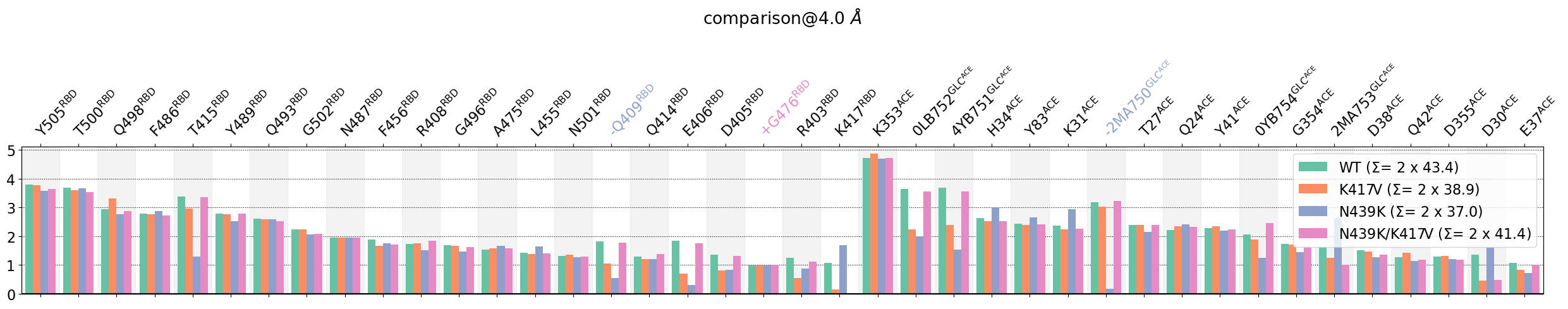
The plot does mainly two things:

• aggregates contact-frequencies per-residue, s.t. bar heights are each residue’s average number of neighbors.

• sorts residues into the [RBD,GLC@RBD]-side or the [ACE,GLC@ACE]-side of the interface.

This immediately informs about the residues that participate the most in the interface between domains, namely, for the RBD: Y505, T500 and for the ACE: K353 (by far). We see also the impact of the mutations, then some glycans, one of them, A2750, severely impacted by the N439K mutation. Other mutation induced changes that can be spotted are the RBD residues K417, E406, and Q409 and K31@ACE.

The legend also informs about the average strength of the interface (=number of residues involved), via the \(\Sigma\) parameter, which is the sum of all the average number of neighbors. We see e.g. the loss of contacts of N439K compared to the WT.

Note:

Please consult the `example notebook <https://proteinformatics.uni-leipzig.de/mdciao/notebooks/Comparing_CGs_Bars.html>`__ devoted to these bar-plot comparisons to read about the \(\Sigma\)-parameter and what meaning can and cannot be extracted from it.

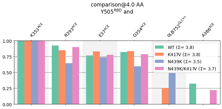
We can take a closer look at these differences by using the `select\_by\_residues <>`__ method of the `ContactGroups <>`__ stored in the interface variable. The method simply creates a new [ContactGroup] with a sub-set of the contacts by using a filtering expression, like "T500"

res = "Y505"
new_CGs = {key: iintf.select_by_residues(res) for key, iintf in interfaces.items()}
mdciao.plots.compare_groups_of_contacts(new_CGs,
                                        ctc_cutoff_Ang=4,
                                        anchor=res,
                                        defrag=None,
                                        colors="Set2",
                                        fontsize=14,
                                       );

These interactions are not shared:
0LB752@GLC^ACE, A386@ACE
Their cumulative ctc freq is 1.28.

Comparing Interfaces: Structures

Next, we are going to use nglviewer and display the ACE-RBD interface in the four setup using the data computed above by mdciao.cli.interface.

Here is what we are doing (and why we are doing it) in the 3D representation.

• Extract a representative geometry/frame with mdciao.contacts.ContactGroup.repframes

  That will locate, for each dataset, the most representative frame (please check to doc to find out what representative means here)
• Save each geometry to a .pdb-file using mdciao.contacts.ContactGroup.frequency_to_bfactor

  This will generate a file that has, as the bfactor for each residue, the bar-heights of the above plot. It essentially paints the 3D structure with an interface-participation heatmap.

• Load these files into an nglview session. Were also doing some other things to ensure the session can be understood better:

• Orient all structures onto the WT representative

• Create four separate, toggeable representations color-coded with bfactor (=interface participation)

  • RBD: cartoon, color-coded in red

  • RBD-interface residues: licorice, color-coded in red

  • ACE: cartoon, color coded in blue

  • ACE-interface residues: licorice, color coded in blue

Note:

The nglviewer visualization can get crowded, and you can choose to visualize the _interface_as_beta.pdb files elsewhere (VMD, pymol, chimera, etc) if the GUI is more intuitive.

Here, however nglviewewr allows us to directly embed the 3D structures into the html documentation directly from the notebook, which is pretty cool.

Feel free to use the widget’s GUI to toggle representations gain insight into the analysis without crowding the picture. Tips:

• View->Full screen

• Hide all components except the WT to begin with, using the eye icon to the right of its name.

• Use the minus/plus / signs to collapse each components’ representations’ menus, the selection string is very distracting.

• Don’t show more than two systems at one, e.g. WT vs K417V or WT vs N439K/K417V.

• For each system, unhide each representation step by step.

ATM it’s not possible to save visualization options into the widget status

Some observations:

• One can see the the respective peaks of the per-residue barplots from above, e.g. Y505@RBD and K353@ACE in very intense red or blue, respectively.

• The ACE glycan with residue numbers in the 750s is also recognizable in blue, as are a number of RBD residues in contact with it in different shades of red, in particular THR415@RBD.

iwd = nglview.NGLWidget()
frags = mdciao.fragments.get_fragments(interfaces["WT"].top,
                                       atoms=True,
                                       verbose=False,
                                       join_fragments=[[0,1],[2,3]], method="chains");
intf_res = [np.unique(np.hstack([iintf.interface_residxs[ii] for iintf in interfaces.values()])) for ii in [0,1]]
colors = ["Reds","Blues"]
repgeoms = {}
for kk, (key, iintf) in enumerate(interfaces.items()):
    repgeoms[key] = iintf.repframes(return_traj=True)[-1][0]
    BB = iintf.top.select("backbone")
    repgeoms[key].superpose(repgeoms["WT"],
                            atom_indices=BB
                           )
    repfile = "%s_interface_as_beta.pdb"%key.replace("/","_")
    iintf.frequency_to_bfactor(4, repfile, repgeoms[key])
    comp = iwd.add_component(nglview.FileStructure(repfile), name=key)


    comp.clear_representations()
    if kk>0:
        visible=False
    else:
        visible=True
    for ii, ifrag in enumerate(frags[:2]):
        intf_atoms = np.hstack([[aa.index for aa in iintf.top.residue(rr).atoms if aa.element.symbol!="H"] for rr in intf_res[ii]])
        rep = comp.add_representation("cartoon",
                               selection=ifrag,
                               colorScheme="bfactor",
                               colorScale=colors[ii],
                               visible=visible,
                              )
        rep = comp.add_representation("licorice",
                                selection=intf_atoms,
                                colorScheme="bfactor",
                                colorScale=colors[ii],
                                visible=visible
                               )

iwd.gui_style = 'ngl'
iwd

Joined Fragments
fragment      0 with    206 AAs   ACE332           (   0) -   0fA738           (205 ) (0)  resSeq jumps
fragment      1 with    767 AAs    ACE18           ( 206) -   0fA796           (972 ) (1)  resSeq jumps
fragment      2 with      2 AAs    CL973           ( 973) -      ZN1           (974 ) (2)  resSeq jumps
fragment      3 with    366 AAs   Na+976           ( 975) -  Na+1341           (1340) (3)
Returning frame 3 of traj nr. 1699: /media/perezheg/6TB_HD/FAH_aws/run3-clone1700.h5

/home/perezheg/miniconda3/lib/python3.8/site-packages/mdtraj/core/trajectory.py:441: UserWarning: top= kwargs ignored since this file parser does not support it
  warnings.warn("top= kwargs ignored since this file parser does not support it")

Contact frequencies stored as bfactor in 'WT_interface_as_beta.pdb'
Returning frame 12 of traj nr. 1345: /media/perezheg/6TB_HD/FAH_aws/run1-clone1345.h5
Contact frequencies stored as bfactor in 'K417V_interface_as_beta.pdb'
Returning frame 3 of traj nr. 269: /media/perezheg/6TB_HD/FAH_aws/run0-clone269.h5
Contact frequencies stored as bfactor in 'N439K_interface_as_beta.pdb'
Returning frame 4 of traj nr. 608: /media/perezheg/6TB_HD/FAH_aws/run2-clone608.h5
Contact frequencies stored as bfactor in 'N439K_K417V_interface_as_beta.pdb'

Comparing Interfaces: Flareplots

Finally, we compare the interfaces using so-called flareplots, using mdciao’s mdciao.flare module, or directly through the higher-level API calls from the [ContactGroup]((http://proteinformatics.uni-leipzig.de/mdciao/api/generated/generated/mdciao.contacts.ContactGroup.html).

Note:

There’s another `entire notebook <http://proteinformatics.uni-leipzig.de/mdciao/notebooks/Comparing_CGs_Flares.html>`__ devoted to how flareplots and flareplot-comparisons can be carried out with with mdciao, and it uses this very same data. You’re highly encouraged to check it out if you want to find out more about the methods and parameters used here.

from matplotlib import pyplot as plt
myfig, myax = plt.subplots(1, 3,sharex=True, sharey=True, figsize=(30,10),
                           tight_layout=True)
frags = mdciao.fragments.get_fragments(interfaces["WT"].top,
                                       verbose=False,
                                       join_fragments=[[0,1],[2,3]], method="chains");
for key, iax in zip(["K417V", "N439K", "N439K/K417V"], myax):
    delta, pairs = interfaces["WT"].frequency_delta(interfaces[key],4)
    mdciao.flare.freqs2flare(delta, pairs,
                             sparse_residues=True,
                             fragments=frags,
                             fragment_names=fragment_names,
                             highlight_residxs=[85,107],
                             signed_colors={-1:"r", +1:"g"},
                             top=interfaces["WT"].top,
                             SS=interfaces[key].repframes(return_traj=True)[-1][0],
                             ax=iax,
                             #subplot=True
                     );
    [iax.plot(np.nan, np.nan, color=col, lw=3, label=key) for key, col in {"formed":"g", "lost":"r"}.items()]
    iax.set_title("%s$\\rightarrow$%s\n$\\Delta \\Sigma = %2.1f$"%("WT",key,delta.sum()),fontsize=30)
    iax.legend(fontsize=20)
myfig.tight_layout()

Joined Fragments
fragment      0 with    206 AAs   ACE332           (   0) -   0fA738           (205 ) (0)  resSeq jumps
fragment      1 with    767 AAs    ACE18           ( 206) -   0fA796           (972 ) (1)  resSeq jumps
fragment      2 with      2 AAs    CL973           ( 973) -      ZN1           (974 ) (2)  resSeq jumps
fragment      3 with    366 AAs   Na+976           ( 975) -  Na+1341           (1340) (3)
Returning frame 12 of traj nr. 1345: /media/perezheg/6TB_HD/FAH_aws/run1-clone1345.h5
Returning frame 3 of traj nr. 269: /media/perezheg/6TB_HD/FAH_aws/run0-clone269.h5
Returning frame 4 of traj nr. 608: /media/perezheg/6TB_HD/FAH_aws/run2-clone608.h5

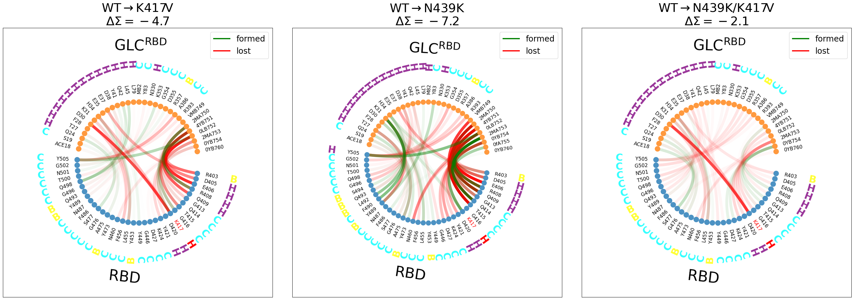
Some observations (it’s better to look at the figure externally with right-click->Open Image in New Tab):

• We have included the \(\Delta\Sigma\) to highlight whether the interface gains or looses contacts upon mutation.

• For WT\(\rightarrow\)K417V (left panel):

• disruption of the K417@RBD-D30@ACE salt-bridge, highlighted in red (also in the the double mutant)

• Y505@RBD loosing contact with ACE and gaining it with ACE’s glycan, although this effect is much stronger in the next panel.

• The RBD-GLC@ACE interface is getting weaker

• For WT\(\rightarrow\)N439 (middle panel):

• Y505@RBD loosing contact with ACE and gaining it with ACE’s glycan

• different interactions between the ACE and RBD are forming: the RBD region L492, F490, Y489 contacts Y83 and K31, both @ACE.

• The ACE glycan loosing some contacts with RBD and/or swapping partner (e.g. T415@ACE for Q414@ACE)

• For WT\(\rightarrow\)N439K/K417V (right panel):

• Disruption of the salt-bridge

• Swapping of interaction partners between RBD and the ACE glycans

You can now go back to the nglviewer locate this individual changes easily.