CLI Tutorial

Basic Usage

Below you will find a very simple example of how to use mdciao from the command-line. Keep scrolling to the Highlights for more elaborate CLI-examples or jump to the Jupyter Notebook for a minimal API walkthrough. For real usecase and some context on definitions etc, go to the Jupyter Notebook Gallery.

Data and 3D visualization

The simulation data for generating these examples was kindly provided by Dr. H. Batebi. It can be 3D-visualized interactively here while checking out the examples. You can also download mdciao_example.zip and follow along.

Copying Terminal Commands

All code snippets can be copied and pasted directly into your terminal using the copy icon in the upper right of the snippet’s frame:

>>> Click the button at end of the frame to copy this text ;)

This basic command:

mdc_neighborhoods.py top.pdb traj.xtc --residues L394 -nf #nf: don't use fragments

will print the following to the terminal (some headers have been left out):

...
The following 6 contacts capture 5.26 (~97%) of the total frequency 5.43 (over 9 contacts with nonzero frequency at 4.50 Angstrom).
[...]
   freq          label            residues  fragments   sum
1  1.00  L394@frag0 - L388@frag0  353 - 347    0 - 0   1.00
2  1.00  L394@frag0 - R389@frag0  353 - 348    0 - 0   2.00
3  0.97  L394@frag0 - L230@frag3  353 - 957    0 - 3   2.97
4  0.97  L394@frag0 - R385@frag0  353 - 344    0 - 0   3.94
5  0.80  L394@frag0 - I233@frag3  353 - 960    0 - 3   4.74
6  0.52  L394@frag0 - K270@frag3  353 - 972    0 - 3   5.26
The following files have been created:
./neighborhood.overall@4.5_Ang.pdf
./neighborhood.LEU394@frag0@4.5_Ang.dat
./neighborhood.LEU394@frag0.time_trace@4.5_Ang.pdf

produce the following figures (not the captions):

_images/neighborhood.overall%404.5_Ang.Fig.1.png — Fig. 1 [`neighborhood.overall@4.5_Ang.pdf`] Using 4.5 Å as distance cutoff, the most frequent neighbors of LEU394, the C-terminal residue in the \(\alpha_5\) helix of the Gs-protein, are shown. \(\Sigma\) is the sum over frequencies and represents the average number of neighbors of LEU394. The simulation started from the 3SN6 structure (beta2 adrenergic receptor-Gs protein complex, no antibody). The simulation itself can be seen interactively in 3D here.

Annotated figures with the timetraces of the above distances are also produced automatically:

_images/neighborhood.LEU394.time_trace%404.5_Ang.Fig.2.png — Fig. 2 [`neighborhood.LEU394.time_trace@4.5_Ang.pdf`] Time-traces of the residue-residue distances used for the frequencies in Fig. 1. The last time-trace represents the total number of neighbors (\(\Sigma\)) within the given cutoff at any given moment in the trajectory. On average, LEU394 has around 4 non-bonded neighbors below the cutoff (see legend of Fig. 1).

Anything that gets shown in any way to the output can be saved for later use as human readable ASCII-files (.dat,.txt), spreadsheets (.ods,.xlsx) or NumPy (.npy) files.

Command Line Tools

The best way to find out about all of mdciao’s command-line tools is to use a command-line tool shipped with mdciao:

>>> mdc_examples.py
usage: mdc_examples.py [-h] [-x] [--short_options] clt

Wrapper script to showcase and optionally run examples of the
command-line-tools that ship with mdciao.

Available command line tools are:
 * mdc_GPCR_overview.py
 * mdc_CGN_overview.py
 * mdc_compare.py
 * mdc_fragments.py
 * mdc_interface.py
 * mdc_neighborhoods.py
 * mdc_pdb.py
 * mdc_residues.py
 * mdc_sites.py

You can type for example:
 > mdc_interface.py  -h
 to view the command's documentation or
 > mdc_examples.py interf
 to show and/or run an example of that command

What these tools do is:

mdc_neighborhoods
Analyse residue neighborhoods using a distance cutoff. Example in Fig. 3.
mdc_interface
Analyse interfaces between any two groups of residues using a distance cutoff. Example here with Fig. 4, Fig. 5, and Fig. 6, among others.
mdc_sites
Analyse a specific set of residue-residue contacts using a distance cutoff. Example in Fig. 8.
mdc_fragments
Break a molecular topology into fragments using different heuristics. Example here.
mdc_GPCR_overview
Map a consensus GPCR nomenclature (e.g. Ballesteros-Weinstein and others) nomenclature on an input topology. Example here.
mdc_CGN_overview
Map a Common G-alpha Numbering (CGN)-type nomenclature on an input topology Example here.
mdc_compare
Compare residue-residue contact frequencies from different files. Example here with Fig. 9.
mdc_pdb
Lookup a four-letter PDB-code in the RCSB PDB and save it locally. Example here.
mdc_residues
Find residues in an input topology using Unix filename pattern matching. Example here.

You can see their documentation by using the -h flag when invoking them from the command line, keep reading the Highlights or the CLI Reference.

Highlights

paper-ready tables and figures from the command line:
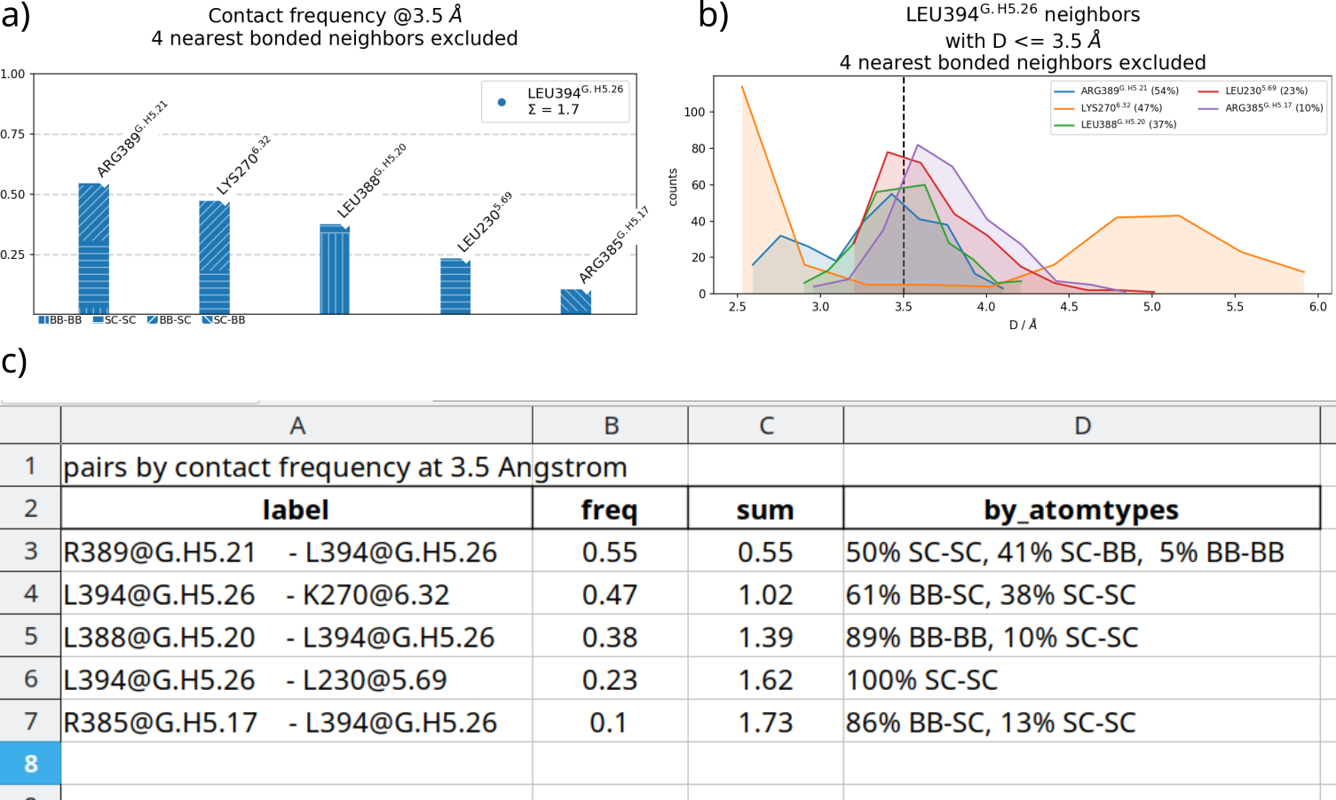
```
mdc_neighborhoods.py top.pdb traj.xtc -r L394 --GPCR adrb2_human --CGN gnas2_human -ni -at #ni: not interactive, at: show atom-types
```
Fig. 3 (click to enlarge) a) contact frequencies for LEU394, as in Fig. 1, but annotated with consensus nomenclature and atom types (--GPCR,--CGN,-at options, see below). b) associated distance distributions, obtained by adding the -d flag to the CLI call. c) Automatically generated table using the -tx xlsx option.

automagically map and incorporate consensus nomenclature to the analysis, either from local files or over the network in the GPRC.db and/or KLIFS:

...
No local file ./adrb2_human.xlsx found, checking online in
https://gpcrdb.org/services/residues/extended/adrb2_human ...done!
Please cite the following reference to the GPCRdb:
 * Kooistra et al, (2021) GPCRdb in 2021: Integrating GPCR sequence, structure and function
   Nucleic Acids Research 49, D335--D343
   https://doi.org/10.1093/nar/gkaa1080
For more information, call mdciao.nomenclature.references()
The GPCR-labels align best with fragments: [3] (first-last: GLU30-LEU340).
Mapping the GPCR fragments onto your topology:
    TM1 with     32 AAs    GLU30@1.29x29   ( 760) -    PHE61@1.60x60   (791 ) (TM1)
   ICL1 with      4 AAs    GLU62@12.48x48  ( 792) -    GLN65@12.51x51  (795 ) (ICL1)
    TM2 with     32 AAs    THR66@2.37x37   ( 796) -    LYS97@2.68x67   (827 ) (TM2)
   ECL1 with      4 AAs    MET98@23.49x49  ( 828) -   PHE101@23.52x52  (831 ) (ECL1)
    TM3 with     36 AAs   GLY102@3.21x21   ( 832) -   SER137@3.56x56   (867 ) (TM3)
   ICL2 with      8 AAs   PRO138@34.50x50  ( 868) -   LEU145@34.57x57  (875 ) (ICL2)
    TM4 with     27 AAs   THR146@4.38x38   ( 876) -   HIS172@4.64x64   (902 ) (TM4)
   ECL2 with     20 AAs   TRP173           ( 903) -   THR195           (922 ) (ECL2)  resSeq jumps
    TM5 with     42 AAs   ASN196@5.35x36   ( 923) -   GLU237@5.76x76   (964 ) (TM5)
   ICL3 with      1 AAs   GLY238           ( 965) -   ARG239           (966 ) (ICL3)
    TM5 with     35 AAs   CYS265@6.27x27   ( 967) -   GLN299@6.61x61   (1001) (TM6)
   ECL2 with      4 AAs   ASP300           (1002) -   ILE303           (1005) (ECL3)
    TM7 with     25 AAs   ARG304@7.31x30   (1006) -   ARG328@7.55x55   (1030) (TM7)
     H8 with     12 AAs   SER329@8.47x47   (1031) -   LEU340@8.58x58   (1042) (H8)
...
Please cite the following reference to the CGN nomenclature:
 * Flock et al, (2015) Universal allosteric mechanism for G$\alpha$ activation by GPCRs
   Nature 2015 524:7564 524, 173--179
   https://doi.org/10.1038/nature14663
For more information, call mdciao.nomenclature.references()
The CGN-labels align best with fragments: [0] (first-last: LEU4-LEU394).
Mapping the CGN fragments onto your topology:
   G.HN with     33 AAs     LEU4@G.HN.10   (   0) -    VAL36@G.HN.53   (32  ) (G.HN)
 G.hns1 with      3 AAs    TYR37@G.hns1.01 (  33) -    ALA39@G.hns1.03 (35  ) (G.hns1)
   G.S1 with      7 AAs    THR40@G.S1.01   (  36) -    LEU46@G.S1.07   (42  ) (G.S1)
...
 G.hgh4 with     21 AAs   TYR311@G.hgh4.01 ( 270) -   ASP331@G.hgh4.21 (290 ) (G.hgh4)
   G.H4 with     16 AAs   PRO332@G.H4.01   ( 291) -   ARG347@G.H4.17   (306 ) (G.H4)
 G.h4s6 with     11 AAs   ILE348@G.h4s6.01 ( 307) -   TYR358@G.h4s6.20 (317 ) (G.h4s6)
   G.S6 with      5 AAs   CYS359@G.S6.01   ( 318) -   PHE363@G.S6.05   (322 ) (G.S6)
 G.s6h5 with      5 AAs   THR364@G.s6h5.01 ( 323) -   ASP368@G.s6h5.05 (327 ) (G.s6h5)
   G.H5 with     26 AAs   THR369@G.H5.01   ( 328) -   LEU394@G.H5.26   (353 ) (G.H5)
...

easy residue selection, with an extended UNIX-like pattern matching. You can preview residue selections like GLU,P0G,3.50,380-394,G.HN.*, which means:
- GLU*: all GLUs, equivalent to GLU
- P0G: the B2AR ligand (agonist)
- 3.50: generic-residue numbering for GPCRs
- 380-394: range of residues with sequence indices 380 to 394 (both incl.). This is the \(G\alpha_5\)-subunit.
- G.HN.* : CGN-nomenclature for the \(G\alpha_N\)-subunit

You can check your selection before running a computation by using mdc_residues.py:

>>> mdc_residues.py GLU*,P0G,380-394,G.HN.* top.pdb --GPCR adrb2_human --CGN GNAS2_HUMAN -ni
Your selection 'GLU*,P0G,380-394,G.HN.*' yields:
   residue      residx    fragment      resSeq        GPCR         CGN
     GLU10           6           0          10        None     G.HN.27
     GLU15          11           0          15        None     G.HN.32
...
    GLU306        1008           3         306     7.33x32        None
    GLU338        1040           3         338     8.56x56        None
    P0G395        1043           4         395        None        None
    ARG380         339           0         380        None     G.H5.12
    ASP381         340           0         381        None     G.H5.13
...
    LEU393         352           0         393        None     G.H5.25
    LEU394         353           0         394        None     G.H5.26
      LEU4           0           0           4        None     G.HN.10
      GLY5           1           0           5        None     G.HN.11
      ASN6           2           0           6        None     G.HN.22
...
     GLN35          31           0          35        None     G.HN.52
     VAL36          32           0          36        None     G.HN.53

easy grabbing structures from the RSC PDB:

>>> mdc_pdb.py 3SN6 -o 3SN6.gro

Checking https://files.rcsb.org/download/3SN6.pdb ...done
Saving to 3SN6.gro...done
Please cite the following 3rd party publication:
 * Crystal structure of the beta2 adrenergic receptor-Gs protein complex
  Rasmussen, S.G. et al., Nature 2011
  https://doi.org/10.1038/nature10361

fragmentation heuristics to easily identify molecules and/or molecular fragments. These heuristics will work on .pdf-files lacking TER and CONNECT records or other file formats, like .gro files, that simply don’t include these records:

Auto-detected fragments with method 'lig_resSeq+'
fragment      0 with  349 AAs     THR9           (   0) -   LEU394           (348 ) (0)  resSeq jumps
fragment      1 with  340 AAs     GLN1           ( 349) -   ASN340           (688 ) (1)
fragment      2 with   58 AAs     ASN5           ( 689) -    ARG62           (746 ) (2)
fragment      3 with  159 AAs  ASN1002           ( 747) -  ALA1160           (905 ) (3)
fragment      4 with  284 AAs    GLU30           ( 906) -   CYS341           (1189) (4)  resSeq jumps
fragment      5 with  128 AAs     GLN1           (1190) -   SER128           (1317) (5)
fragment      6 with    1 AAs  P0G1601           (1318) -  P0G1601           (1318) (6)

In this example, we saved the crystal structure 3SN6 as a .gro-file (mdc_pdb.py 3SN6 -o 3SN6.gro). We are able to recover sensible fragments:

\(G\alpha\)
\(G\beta\)
\(G\gamma\)
bacteriophage T4 lysozyme as N-terminus of the receptor (next)
\(\beta 2\) adrenergic receptor
VHH antibody
ligand.

For clarity, we omitted the fragmentation in our initial example with the option -nf, but all CLI tools do this fragmentation by default. Alternatively, one can use:

mdc_fragments.py 3SN6.gro

to get an overview of all available fragmentation heuristics and their results without computing any contacts whatsoever.

use fragment definitions –like the ones above, 0 for the \(G\alpha\)-unit and 3 for the receptor– to compute interfaces in an automated way, i.e. without having to specifying individual residues:

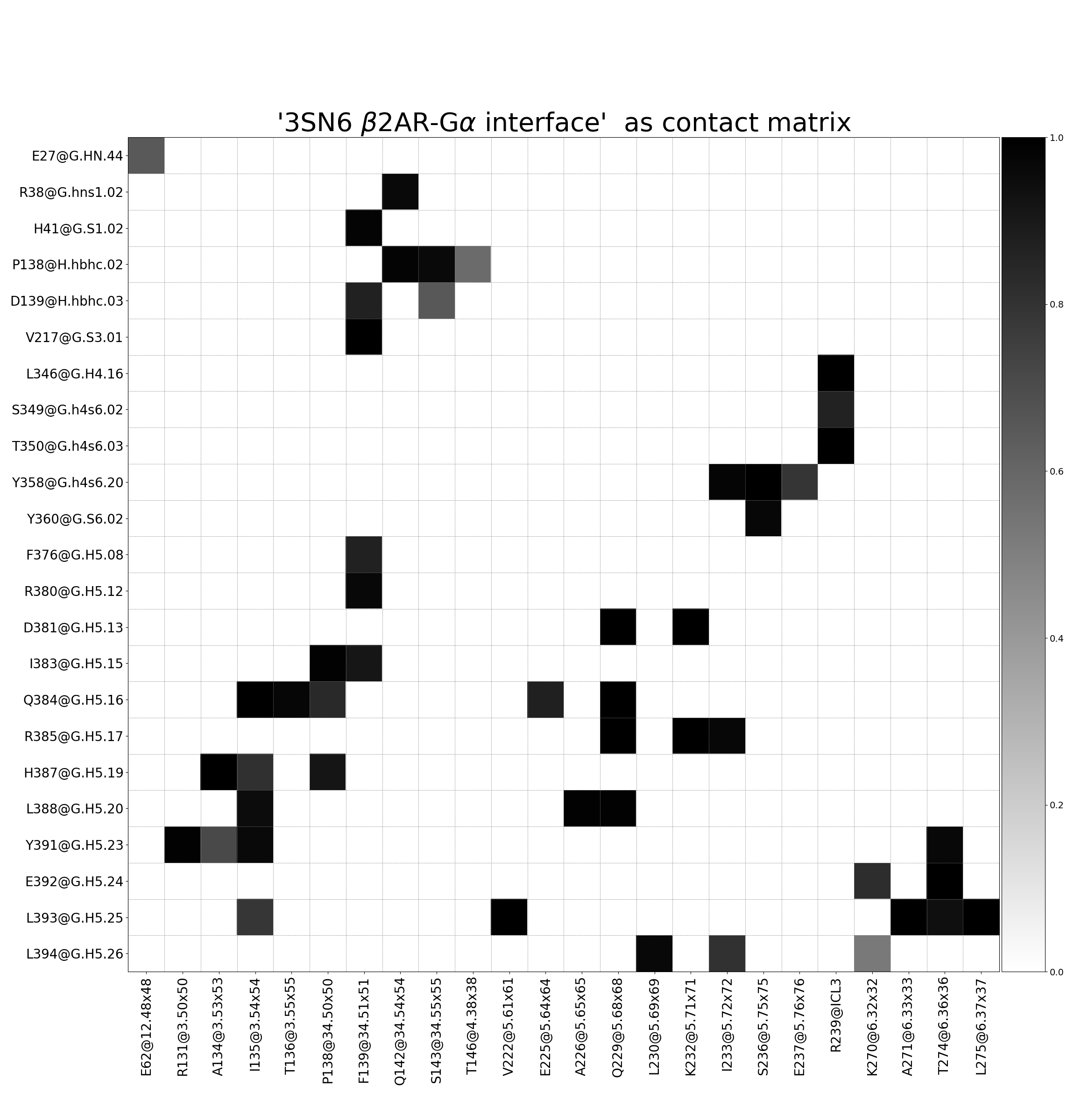
>>> mdc_interface.py top.pdb traj.xtc -isel1 0 -isel2 3 --GPCR adrb2_human --CGN gnas2_human -t "3SN6 beta2AR-Galpha interface" -ni
...
The following 50 contacts capture 45.66 (~91%) of the total frequency 50.28 (over 107 contacts with nonzero frequency at 4.50 Angstrom).
As orientation value, the first 50 ctcs already capture 90.0% of 50.28.
The 50-th contact has a frequency of 0.52.

    freq              label               residues  fragments   sum
1   1.00  R385@G.H5.17   - K232@5.71x71   344 - 959    0 - 3    1.00
2   1.00  V217@G.S3.01   - F139@34.51x51  183 - 869    0 - 3    2.00
3   1.00  R385@G.H5.17   - Q229@5.68x68   344 - 956    0 - 3    3.00
4   1.00  D381@G.H5.13   - Q229@5.68x68   340 - 956    0 - 3    4.00
5   1.00  E392@G.H5.24   - T274@6.36x36   351 - 976    0 - 3    5.00
6   1.00  Y358@G.h4s6.20 - S236@5.75x75   317 - 963    0 - 3    6.00
7   1.00  D381@G.H5.13   - K232@5.71x71   340 - 959    0 - 3    7.00
...
./interface.overall@4.5_Ang.xlsx
./interface.overall@4.5_Ang.dat
./interface.overall@4.5_Ang.as_bfactors.pdb
./interface.overall@4.5_Ang.pdf
./interface.matrix@4.5_Ang.pdf
./interface.flare@4.5_Ang.pdf
./interface.time_trace@4.5_Ang.pdf

Fig. 4 [interface.matrix@4.5_Ang.pdf](click to enlarge). Interface contact matrix between the β2AR receptor and the α-unit of the G-protein, using a cutoff of 4.5 Å. The labelling incorporates consensus nomenclature to identify positions and domains of both receptor and G-protein. Please note: this is not a symmetric contact-matrix. The y-axis shows residues in the Gα-unit and the x-axis in the receptor.

Since Fig. 4 is bound to incorporate a lot of blank pixels, mdciao will also produce sparse plots and figures that highlight the formed contacts only:

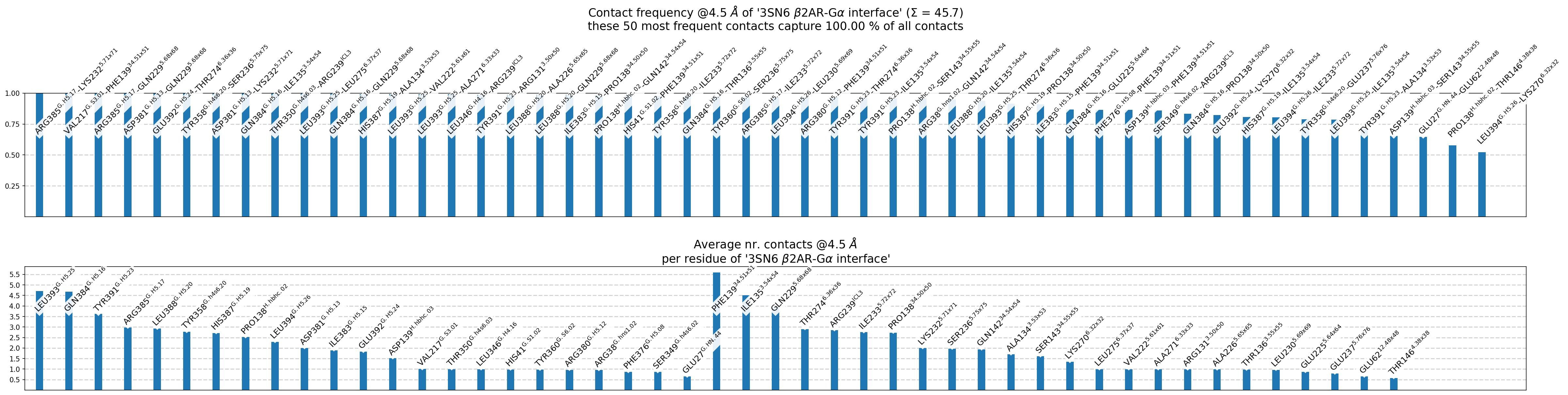
Fig. 5 [interface.overall@4.5_Ang.pdf](click to enlarge) Upper panel: most frequent contacts sorted by frequency, i.e. for each non-empty pixel of Fig. 4, there is a bar shown. Lower panel: per-residue aggregated contact-frequencies, showing each residue’s average participation in the interface (same info will be written to interface.overall@4.5_Ang.xlsx). Also, the number of shown contacts/bars can be controlled either with the –ctc_control and/or –min_freq parameters of mdc_interface.py.

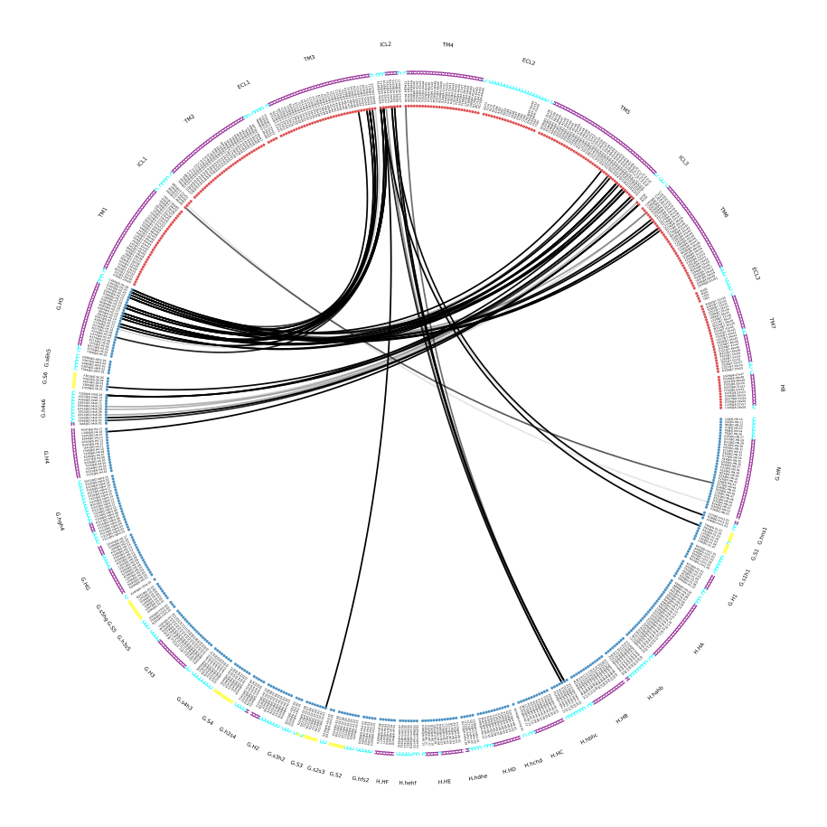
A very convenient way to incorporate the molecular topology into the visualization of contact frequencies are the so-called FlarePlots (cool live-demo here). These show the molecular topology (residues, fragments) on a circle with curves connecting the residues for which a given frequency has been computed. mdciao has its own flareplot implementation in the mdciao.flare module, that can also coarse-grain flareplots to the molecular fragments. The mdc_interface.py example above will generates a flareplot by default:

Fig. 6 [interface.flare@4.5_Ang.pdf](click to enlarge) FlarePlot of the frequencies shown in the figures Fig. 4 and Fig. 5. Residues are shown as dots on a circumference, split into fragments following any available labelling information. The contact frequencies are represented as lines connecting these dots/residues, with the line-opacity proportional to the frequencie’s value. The secondary stucture of each residue is also included as color-coded letters: H(elix), B(eta), C(oil). We can clearly see the \(G\alpha_5\)-subunit in contact with the receptor’s TM3, ICL2, and TM5-ICL3-TM6 regions. Note that this plot is always produced as .pdf to be able to zoom into it as much as needed.

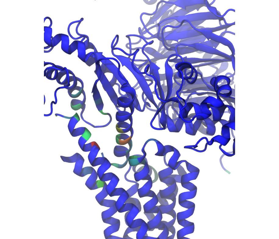
Similar to how the flareplot (Fig. 6) is mapping contact-frequencies (Fig. 5, upper panel) onto the molecular topology, the next figure maps the lower panel Fig. 5 on the molecular geometry. It simply puts the values shown there in the temperature factor of a pdb file, representing the calculated interface as a heatmap, which can be visualized in VMD using the Beta coloring.

Fig. 7 [interface.overall@4.5_Ang.as_bfactors.pdb](click to enlarge) 3D visualization of the interface as heatmap (blue-green-red) using VMD. We clearly see the regions noted in Fig. 6 (TM5-ICL3-TM6 and \(G\alpha_5\)-subunit) in particular the residues of Fig. 5 (lower panel) light up. This heatmap is overlaid on structures representative of the interface, and have been selected using the mdciao.contacts.ContactGroup.repframes method. Please note, for the homepage-banner (red-blue heatmap), the signed_colors argument has been used when calling the mdciao.flare.freqs2flare method of the API. At the moment this is not possible just by using mdc_interface.py, sorry!

You can use this snippet to generate a VMD visualiazation state file, view_mdciao_interface.vmd to view the heatmap:
echo 'mol new ./interface.overall@4.5_Ang.as_bfactors.pdb
      mol modstyle 0 0 NewCartoon
      mol modcolor 0 0 Beta
      color scale method BGR ' > view_mdciao_interface.vmd
vmd -e view_mdciao_interface.vmd
view_mdciao_interface.vmd will work with any *.as_bfactors.pdb file that mdciao generates. For our example, you can also paste this viewpoint into your VMD console and generate a view equivalent to the above picture (results may vary with other files):
molinfo top set {center_matrix rotate_matrix scale_matrix global_matrix} {{{1 0 0 -66.7954} {0 1 0 -66.6322} {0 0 1 -45.2629} {0 0 0 1}} {{-0.688392 0.720507 0.0835694 0} {-0.0925729 0.0269995 -0.995339 0} {-0.719405 -0.692919 0.0481138 0} {0 0 0 1}} {{0.0348044 0 0 0} {0 0.0348044 0 0} {0 0 0.0348044 0} {0 0 0 1}} {{1 0 0 0.15} {0 1 0 0.12} {0 0 1 0} {0 0 0 1}}}

A different approach is to look only for a particular set of pre-defined contacts. Simply writing this set into a human readable JSON file will allow mdc_sites.py to compute and present these (and only these) contacts, as in the example file tip.json:
```
>>> echo '
>>> {"name":"interface small",
>>> "pairs": {"AAresSeq": [
>>>         "L394-K270",
>>>         "D381-Q229",
>>>         "Q384-Q229",
>>>         "R385-Q229",
>>>         "D381-K232",
>>>         "Q384-I135"
>>>         ]}}' > tip.json
```
One added bonus is that the same .json files can be used file across different setups as long as the specified residues are present.

The command:
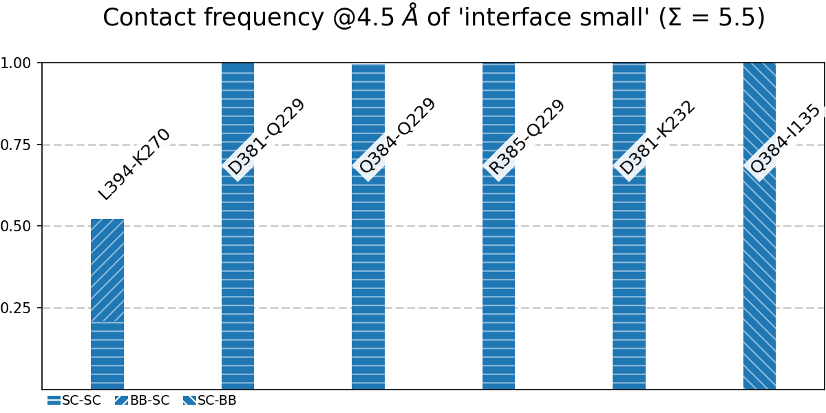
```
>>> mdc_sites.py top.pdb traj.xtc --site tip.json -at -nf -sa #sa: short AA-names
...
The following files have been created:
./sites.overall@4.5_Ang.pdf
...
```
generates the following figure (tables are generated but not shown). The option -at (--atomtypes) generates the patterns (“hatching”) of the bars. They indicate what atom types (sidechain or backbone) are responsible for the contact:

Fig. 8 [sites.overall@4.5_Ang.pdf](click to enlarge) Contact frequencies of the residue pairs specified in the file tip.json, shown with the contact type indicated by the stripes on the bars. Use e.g. the 3D-visualisation to check how “L394-K270” switches between SC-SC and SC-BB.

compare contact frequencies coming from different calculations, to detect and show contact changes across different systems. For example, to look for the effect of different ligands, mutations, pH-values etc. In this case, we compare the neighborhood of R131 (3.50 on the receptor) between our MD simulations and the crystal structure straight from the PDB. First, we grab the file on the fly with mdc_pdb.py:

>>> mdc_pdb.py 3SN6
Checking https://files.rcsb.org/download/3SN6.pdb ...done
Saving to 3SN6.pdb...done
Please cite the following 3rd party publication:
 * Crystal structure of the beta2 adrenergic receptor-Gs protein complex
   Rasmussen, S.G. et al., Nature 2011
   https://doi.org/10.1038/nature10361

Now we use mdc_neighborhoods.py on it:

>>> mdc_neighborhoods.py 3SN6.pdb 3SN6.pdb -r R131 -o 3SN6 -nf -o 3SN6.X
...
The following 5 contacts capture 5.00 (~100%) of the total frequency 5.00 (over 5 contacts with nonzero frequency at 4.50 Angstrom).
As orientation value, the first 5 ctcs already capture 90.0% of 5.00.
The 5-th contact has a frequency of 1.00.
   freq    label       residues   fragments  sum
1   1.0  R131 - Y326  1007 - 1174    0 - 0   1.0
2   1.0  R131 - Y391   1007 - 345    0 - 0   2.0
3   1.0  R131 - V222  1007 - 1095    0 - 0   3.0
4   1.0  R131 - Y219  1007 - 1092    0 - 0   4.0
5   1.0  R131 - I278  1007 - 1126    0 - 0   5.0
The following files have been created:
./3SN6.X.ARG131@4.5_Ang.dat

Now we use mdc_neighborhoods.py on our data:

>>> mdc_neighborhoods.py top.pdb traj.xtc -r R131 -nf -o 3SN6.MD
...
The following 6 contacts capture 3.15 (~99%) of the total frequency 3.17 (over 7 contacts with nonzero frequency at 4.50 Angstrom).
As orientation value, the first 4 ctcs already capture 90.0% of 3.17.
The 4-th contact has a frequency of 0.39.
   freq    label       residues  fragments   sum
1  0.99  R131 - Y391   861 - 350    0 - 0   0.99
2  0.94  R131 - Y326  861 - 1028    0 - 0   1.92
3  0.76  R131 - Y219   861 - 946    0 - 0   2.69
4  0.39  R131 - I278   861 - 980    0 - 0   3.07
5  0.05  R131 - I325  861 - 1027    0 - 0   3.12
6  0.02  R131 - I72    861 - 802    0 - 0   3.15

...
The following files have been created:
...
./3SN6.MD.ARG131@4.5_Ang.dat

Please note that we have omitted most of the terminal output, and that we have used the option -o to label output-files differently: 3SN6.X and 3SN6.MD. Now we compare both these outputs:
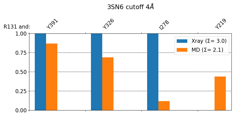
>>> mdc_compare.py 3SN6.X.ARG131@4.5_Ang.dat 3SN6.MD.ARG131@4.5_Ang.dat -k Xray,MD -t "3SN6 cutoff 4.5AA" -a R131
These interactions are not shared:
I325, I72, V222
Their cumulative ctc freq is 1.07.
Created files
freq_comparison.pdf
freq_comparison.xlsx
Fig. 9 [freq_comparison.pdf]Neighborhood comparison for R131 between our MD simulations and the original 3SN6 crystal structure. We can see how the neighborhood relaxes and changes. Some close residues, in particular I278, move further than 4.5 Å away from R131. You can see these residues highlighted in the 3D visualization. We have used a custom title and custom keys for clarity of the figure (options -t and -k). Also, since all contact labels share the ‘R131’ label, we can remove it with the -a (anchor residue).

API

The API is what you get to your Python scope upon importing mdciao, .e.g.:

import mdciao

The API has a dedicated submodule to replicate the Command-Line-Interface, mdciao.cli and a lot of other methods that expose useful functions to create your own workflows. The the Jupyter Notebook Tutorial has some highlights and easy walkthroughs, while the Jupyter Notebook Gallery for some more fancy examples. Check the API Reference page for the full API documentation.

Note

Whereas the command-line-tools tend to be more stable, the API might experience some minor changes until the first major release.