Comparing Frequencies: Consensus Nomenclature
In this notebook, we exploit the GPCR consensus nomenclature to compute and compare contact frequencies across four GPCRs that have very little sequence identity.
Nevertheless, the consensus nomenclature will allow us to:
Use the same function calls for all systems, regardless of the underlying primary sequence
Compare the frequencies across systems by using consensus labels
- Growth hormone secretagogue receptor type 1, ghrelin receptor for short.Provided kindly by Dr. A. Vogel
- Neuropeptide Y receptor type 1, Y1 receptor for short, in apo form.Provided kindly by Dr. A. Vogel.
- Active mu-opioid receptor bound to the agonist morphine.Kindly made available for this purpose by the GPCRmd.
All these example datasets will be downloaded on the fly using mdciao.examples.fetch_example_data, please note the individual references for each dataset there.
Also note that mdciao ships with all references regarding the used nomenclature schemes, you can issue mdciao.nomenclature.references to print them out.
[1]:
import mdciao
Download Trajectory Data
Throughout the notebook, we will use the same aliases used by mdciao.examples.fetch_example_data to adress the different sytems/datasets, "b2ar@Gs", "ghrelin@ghsr" , "mor@muor", "y1_apo", but one could create an alias dictionary for nicer tagging of plots etc (see note at the bottom of the notebook).
[2]:
systems = ["b2ar@Gs",
"ghrelin@ghsr" ,
"mor@muor",
"y1_apo"]
for system in systems:
d = mdciao.examples.fetch_example_data(system,
unzip=system,
skip_on_existing=True)
Unzipping to 'b2ar@Gs'
Unzipping to 'ghrelin@ghsr'
Unzipping to 'mor@muor'
Unzipping to 'y1_apo'
Nomenclature Data
We will get the nomenclature data, i.e. the per-residue consensus labels mapped to the canonical primary sequence of the receptor, from the GPCRdb (in this case). The lookup happens via UniProt Entry Names and uses mdciao’s nomenclature clases.
These objects contain all nomenclature information, and map the consensus labels and fragments (“3.50”, or “TM3”, respectively) not only to the canonical sequence, but to tht of the topologies at hand, using class methods like top2labels and top2frags.
So, as a user, you need to know these UniProt Entry Names for each one of your systems.
[3]:
key2GPCR_UniProt = {"b2ar@Gs" : "adrb2_human",
"ghrelin@ghsr" : "ghsr_human",
"mor@muor" : "oprm_mouse",
"y1_apo" : "npy1r_human"
}
GPCR = {key : mdciao.nomenclature.LabelerGPCR(val, scheme="BW",
write_to_disk=True, local_path=key) for key, val in key2GPCR_UniProt.items()}
No local file b2ar@Gs/adrb2_human.xlsx found, checking online in
https://gpcrdb.org/services/residues/extended/adrb2_human ...done!
Please cite the following reference to the GPCRdb:
* Kooistra et al, (2021) GPCRdb in 2021: Integrating GPCR sequence, structure and function
Nucleic Acids Research 49, D335--D343
https://doi.org/10.1093/nar/gkaa1080
For more information, call mdciao.nomenclature.references()
wrote b2ar@Gs/adrb2_human.xlsx for future use
No local file ghrelin@ghsr/ghsr_human.xlsx found, checking online in
https://gpcrdb.org/services/residues/extended/ghsr_human ...done!
Please cite the following reference to the GPCRdb:
* Kooistra et al, (2021) GPCRdb in 2021: Integrating GPCR sequence, structure and function
Nucleic Acids Research 49, D335--D343
https://doi.org/10.1093/nar/gkaa1080
For more information, call mdciao.nomenclature.references()
wrote ghrelin@ghsr/ghsr_human.xlsx for future use
No local file mor@muor/oprm_mouse.xlsx found, checking online in
https://gpcrdb.org/services/residues/extended/oprm_mouse ...done!
Please cite the following reference to the GPCRdb:
* Kooistra et al, (2021) GPCRdb in 2021: Integrating GPCR sequence, structure and function
Nucleic Acids Research 49, D335--D343
https://doi.org/10.1093/nar/gkaa1080
For more information, call mdciao.nomenclature.references()
wrote mor@muor/oprm_mouse.xlsx for future use
No local file y1_apo/npy1r_human.xlsx found, checking online in
https://gpcrdb.org/services/residues/extended/npy1r_human ...done!
Please cite the following reference to the GPCRdb:
* Kooistra et al, (2021) GPCRdb in 2021: Integrating GPCR sequence, structure and function
Nucleic Acids Research 49, D335--D343
https://doi.org/10.1093/nar/gkaa1080
For more information, call mdciao.nomenclature.references()
wrote y1_apo/npy1r_human.xlsx for future use
For the "b2ar@Gs system, we also get the CGN labels, i.e. those for the G-protein.
[4]:
CGN = {"b2ar@Gs" : mdciao.nomenclature.LabelerCGN("gnas2_human", write_to_disk=True, local_path="b2ar@Gs")}
No local file b2ar@Gs/gnas2_human.xlsx found, checking online in
https://gpcrdb.org/services/residues/extended/gnas2_human ...done!
Please cite the following reference to the GPCRdb:
* Kooistra et al, (2021) GPCRdb in 2021: Integrating GPCR sequence, structure and function
Nucleic Acids Research 49, D335--D343
https://doi.org/10.1093/nar/gkaa1080
Please cite the following reference to the CGN nomenclature:
* Flock et al, (2015) Universal allosteric mechanism for G$\alpha$ activation by GPCRs
Nature 2015 524:7564 524, 173--179
https://doi.org/10.1038/nature14663
For more information, call mdciao.nomenclature.references()
wrote b2ar@Gs/gnas2_human.xlsx for future use
Note that in the above cells we’re storing the retrieved data as .xlsx-files in the individual directories.
Residue Neighborhood of 3.50
We start by computing the residue neighborhood of notorious residue 3.50 of TM3 in all systems, without even knowing what residue precisely is 3.50 in all systems.
Since we will store the results in the rn dictionary and compare them across systems later, we’re supressing all outputs in the cell below, but feel free to comment out the %%capture and the #figures=False statements
[5]:
%%capture
rn = {}
for system in systems:
rn[system] = list(mdciao.cli.residue_neighborhoods("3.50", f"{system}/traj.xtc", topology=f"{system}/top.pdb",
output_dir=system, GPCR_UniProt=GPCR[system], accept_guess=True,
ctc_control=1.0,
no_disk=True,
figures=False,
CGN_UniProt=CGN.get(system,None),
fragments="chains").values())[0]
Compare Frequency Bars
We show all contact frequencies of all four systems together using mdciao.plots.compare_groups_of_contacts.
To show what the plot would look like without the consensus labels, initially we won’t make use of them:
[6]:
fig, ax ,plotted_freqs = mdciao.plots.compare_groups_of_contacts(rn, ctc_cutoff_Ang=4.5,
figsize=(20,5),
defrag=None);
These interactions are not shared:
C146@3.55-R141@3.50, D340@8.47-R165@3.50, E257@6.29-R138@3.50, I234@5.61-R138@3.50, I235@5.61-R141@3.50, I261@6.33-R138@3.50, I278@6.33-R165@3.50, I278@6.40-R131@3.50, I325@7.52-R131@3.50, I72@2.43-R131@3.50, K152@34.54-R141@3.50, K328@8.48-R141@3.50, K329@8.49-R141@3.50, L239@5.65-R141@3.50, L265@6.37-R138@3.50, L323@7.56-R138@3.50, L339@7.56-R165@3.50, L82@2.43-R141@3.50, M244@5.71-R138@3.50, M255@5.61-R165@3.50, M281@6.36-R165@3.50, M326@7.56-R141@3.50, N262@6.34-R138@3.50, R131@3.50-V222@5.61, R131@3.50-Y219@5.58, R131@3.50-Y326@7.53, R131@3.50-Y391@G.H5.23, R138@3.50-T258@6.30, R138@3.50-T75@2.39, R138@3.50-Y231@5.58, R138@3.50-Y253@6.25, R141@3.50-R150@34.52, R141@3.50-S327@8.47, R141@3.50-T76@2.37, R141@3.50-T78@2.39, R141@3.50-Y232@5.58, R141@3.50-Y323@7.53, R141@3.50-Y330@8.50, R165@3.50-R179@34.57, R165@3.50-T103@2.39, R165@3.50-Y106@2.42, R165@3.50-Y252@5.58
Their cumulative ctc freq is 18.11.
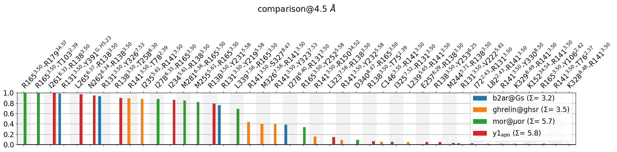
This plot is a mess, since all 3.50 residues are different residues in all systems: * R131 in b2ar@Gs * R141 in ghrelin@ghsr * R165 in mor@muor * R138 in y1_apo
Of course, the same goes for all other residues. This means there’s no shared contact pairs to be compared agains each other when using residue names.
However, if we specifiy AA_format="try_consensus", the method will try to use those labels (which are unified across systems) when possible:
[7]:
fig, ax ,plotted_freqs = mdciao.plots.compare_groups_of_contacts(rn, ctc_cutoff_Ang=4.5, defrag=None,
AA_format="try_consensus",
anchor="3.50",
sort_by="consensus",
);
These interactions are not shared:
2.37, 2.39, 2.42, 2.43, 3.55, 34.52, 34.54, 34.57, 5.65, 5.71, 6.25, 6.29, 6.30, 6.33, 6.34, 6.36, 6.37, 6.40, 7.52, 7.53, 7.56, 8.47, 8.48, 8.49, 8.50, G.H5.23
Their cumulative ctc freq is 13.55.
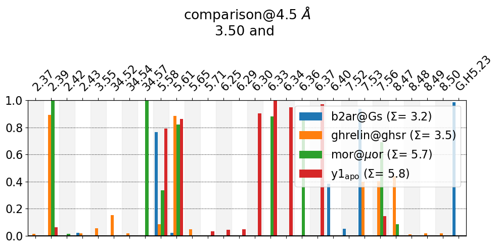
Much nicer. We also make the plot even more compact by using: * anchor="3.50" this eliminates “3.50” from all labels and only uses the label of the other residue in the residue pair. * sort_by="consensus" sorts the contacts, insted of by descending frequency (like the first plot), by their consensus label.
Also note, in b2ar@Gs, one residue corresponds to the Gs-unit, the 23rd residue of the α5 helix.
Interface: TM3 vs all other TMs
We now compute whole interfaces between fragments following the same approach, i.e using consensus labels. In this case, we’re computing the contacts of the TM3 with all other elements of the system. We’re doing so by using the keyword arguments:
interface_selection_1="TM3",
interface_selection_2="*",
For the purposes of this notebook, we focus on the usage of consensus descriptors, but please read the full documentation in mdciao.cli.interface for how interfaces can be defined.
Also note that we’re supressing the output since we will be comparing (like above) the different systems later. Just comment out the %%capture if you want to see the output and the figures. ### Compute
[8]:
%%capture
intf = {}
for system in systems:
intf[system] = mdciao.cli.interface(f"{system}/traj.xtc", topology=f"{system}/top.pdb", output_dir=system,
GPCR_UniProt=GPCR[system],
accept_guess=True,
CGN_UniProt=CGN.get(system, None),
ctc_control=1.0,
interface_selection_1="TM3",
interface_selection_2="*",
no_disk=True,
fragments="chains",
plot_timedep=False,
figures=True,
self_interface=True,
title=f"interface {system}",
n_nearest=4
)
Compare Frequency Bars
Using the same method as above, we compare now frequencies, but instead of resolving to each individual pair (there’s about 150 TM3 vs all contacts), we aggregate the frequencies to each residue using per_residue=True. This loses the per-pair information but makes the plot more compact to begin with.
[9]:
mdciao.plots.plots.compare_groups_of_contacts(intf, ctc_cutoff_Ang=4.5, defrag=None,
per_residue=True,
AA_format="try_consensus",
figsize=None,
sort_by="consensus",
lower_cutoff_val=1,
interface=True,
);
These interactions are not shared:
3.23, 3.56
Their cumulative ctc freq is 2.61.
These interactions are not shared:
2.37, 2.38, 2.50, 2.57, 2.59, 2.61, 2.63, 2.64, 34.50, 34.52, 34.53, 34.55, 34.56, 34.57, 4.38, 4.46, 4.58, 4.60, 4.63, 45.52, 5.38, 5.39, 5.42, 5.43, 5.47, 5.51, 5.65, 5.70, 5.71, 5.72, 6.23, 6.25, 6.29, 6.30, 6.33, 6.34, 6.36, 6.37, 6.40, 6.41, 6.45, 6.48, 6.51, 6.52, 6.55, 7.35, 7.39, 7.42, 7.43, 7.45, 7.46, 7.49, 7.52, 7.53, 7.56, 8.47, C184@ECL2, C190@ECL2, E188@ECL2, G.H5.16, G.H5.19, G.H5.20, G.H5.23, G.H5.25, G1, G183@ECL2, K247@ICL3, M179@ECL2, M248@ICL3, MOR353, P0G395, P150@ICL2, R146@ICL2, R149@ICL2, R175@ECL2, R187@ECL2, S3, T207@ECL2, T208@ECL2, V178@ECL2, V184@ECL2, W148@ICL2, Y174@ECL2, Y185@ECL2
Their cumulative ctc freq is 151.03.

There’s a lot to unpack here, but we we can immediately see that e.g. 3.28 and 3.37 behave differently across systems. We’ll check them later, but now we pick a representation that tries to be compact without losing pair information.
Compare Flareplots
[10]:
from matplotlib import pyplot as plt
myfig, myax = plt.subplots(2,2, sharex=True, sharey=True, figsize=(70,70), tight_layout=True)
for (system, iintf) , iax in zip(intf.items(), myax.flatten()):
consensus_maps=[GPCR[system]]
iCGN = CGN.get(system, None)
if iCGN is not None:
consensus_maps.append(iCGN)
iintf.plot_freqs_as_flareplot(4.5, fragments="chains",
scheme="consensus_sparse",
aura=iintf.frequency_sum_per_residue_idx_dict(4.5, return_array=True),
panelsize=15,
ax=iax,
consensus_maps=consensus_maps)
iax.set_title(f"{system}: TM3 interface at 4.5 Å", fontsize=60)
print()
myfig.tight_layout(h_pad=5)
Auto-detected fragments with method 'chains'
fragment 0 with 354 AAs LEU4 ( 0) - LEU394 (353 ) (0) resSeq jumps
fragment 1 with 340 AAs GLN1 ( 354) - ASN340 (693 ) (1)
fragment 2 with 66 AAs ALA2 ( 694) - PHE67 (759 ) (2)
fragment 3 with 207 AAs GLU30 ( 760) - ARG239 (966 ) (3) resSeq jumps
fragment 4 with 76 AAs CYS265 ( 967) - LEU340 (1042) (4)
fragment 5 with 1 AAs P0G395 (1043) - P0G395 (1043) (5)
Auto-detected fragments with method 'chains'
fragment 0 with 15 AAs GLY1 ( 0) - ARG15 (14 ) (0)
fragment 1 with 308 AAs ASP32 ( 15) - GLY339 (322 ) (1)
Auto-detected fragments with method 'chains'
fragment 0 with 289 AAs SER64 ( 0) - ILE352 (288 ) (0)
fragment 1 with 1 AAs MOR353 ( 289) - MOR353 (289 ) (1)
Auto-detected fragments with method 'chains'
fragment 0 with 321 AAs PHE18 ( 0) - ASP339 (320 ) (0) resSeq jumps
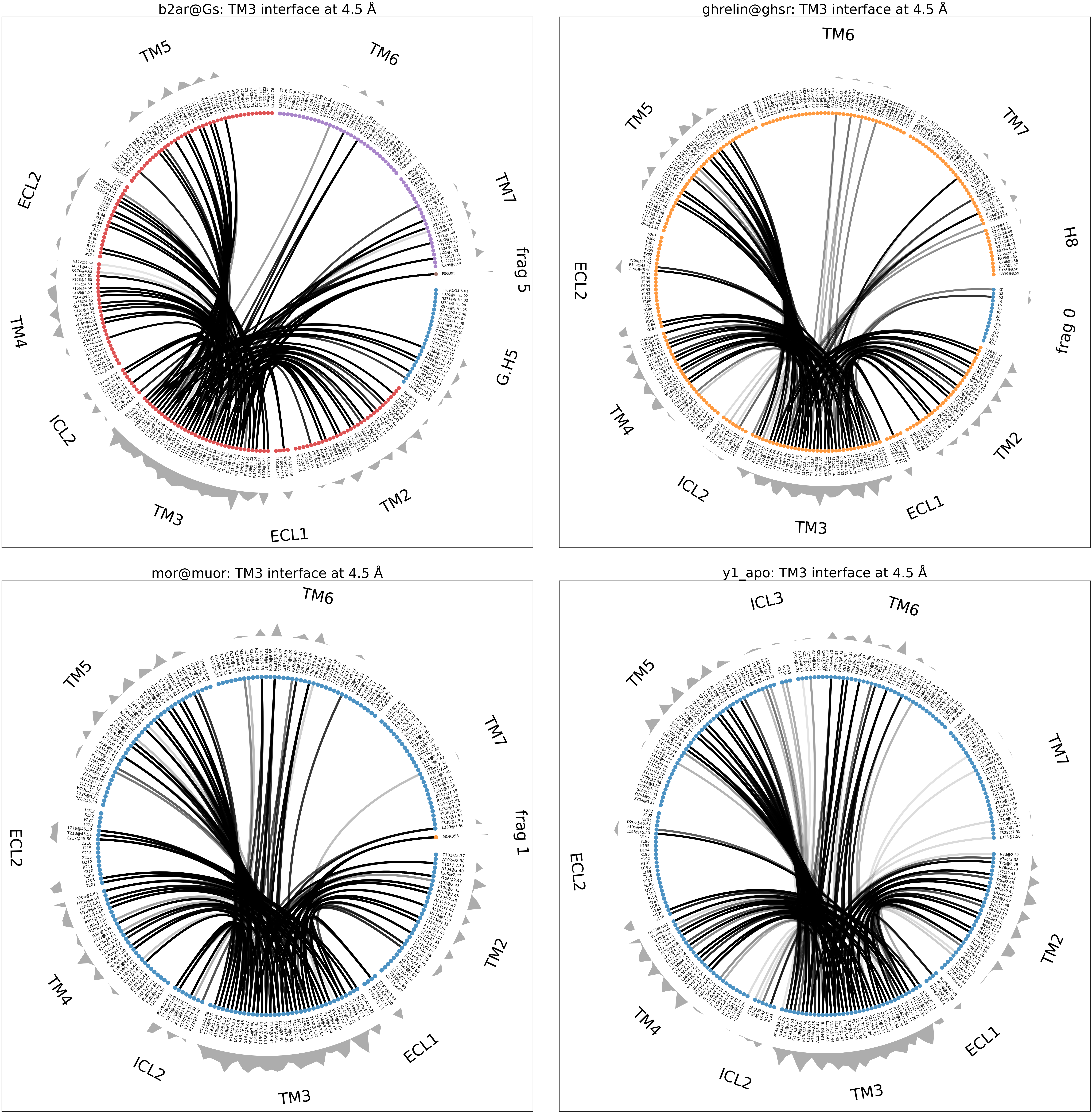
This representation tries to capture the system’s topology, and the individual pairs as well as collective behaviours. We have an `entire notebook <>`__ devoted on how these plots work and how one can fine-tune them. One of the easiest things to spot is the difference in TM3 vs TM6 contacts.
Coarse-Graining to Consensus Fragments
We can also coarse-grain the frequencies to the fragments, showing a bit the structure and scaffolding role of TM3 in the TM-bundle. All this, without having to directly define the fragments for each system:
[11]:
import pandas
CG_freqs = {}
for (system, iintf) , iax in zip(intf.items(), myax.flatten()):
consensus_maps=[GPCR[system]]
iCGN = CGN.get(system, None)
if iCGN is not None:
consensus_maps.append(iCGN)
CG_freqs[system] = iintf.frequency_as_contact_matrix_CG (4.5, fragments=mdciao.fragments.get_fragments(iintf.top, "chains"),
sparse=True,
consensus_labelers=consensus_maps)["TM3"]
df = pandas.DataFrame(CG_freqs).T
df = df[[key for key in mdciao.nomenclature.nomenclature._GPCR_fragments+mdciao.nomenclature.nomenclature._CGN_fragments if key in df.keys()]]
df.round(1).fillna("")
Auto-detected fragments with method 'chains'
fragment 0 with 354 AAs LEU4 ( 0) - LEU394 (353 ) (0) resSeq jumps
fragment 1 with 340 AAs GLN1 ( 354) - ASN340 (693 ) (1)
fragment 2 with 66 AAs ALA2 ( 694) - PHE67 (759 ) (2)
fragment 3 with 207 AAs GLU30 ( 760) - ARG239 (966 ) (3) resSeq jumps
fragment 4 with 76 AAs CYS265 ( 967) - LEU340 (1042) (4)
fragment 5 with 1 AAs P0G395 (1043) - P0G395 (1043) (5)
Auto-detected fragments with method 'chains'
fragment 0 with 15 AAs GLY1 ( 0) - ARG15 (14 ) (0)
fragment 1 with 308 AAs ASP32 ( 15) - GLY339 (322 ) (1)
Auto-detected fragments with method 'chains'
fragment 0 with 289 AAs SER64 ( 0) - ILE352 (288 ) (0)
fragment 1 with 1 AAs MOR353 ( 289) - MOR353 (289 ) (1)
Auto-detected fragments with method 'chains'
fragment 0 with 321 AAs PHE18 ( 0) - ASP339 (320 ) (0) resSeq jumps
[11]:
| TM2 | ECL1 | TM3 | ICL2 | TM4 | ECL2 | TM5 | ICL3 | TM6 | TM7 | H8 | G.H5 | |
|---|---|---|---|---|---|---|---|---|---|---|---|---|
| b2ar@Gs | 27.2 | 3.0 | 0.2 | 7.6 | 23.3 | 12.1 | 23.0 | 4.1 | 8.9 | 8.3 | ||
| ghrelin@ghsr | 27.3 | 2.9 | 0.2 | 1.3 | 27.6 | 8.1 | 25.7 | 2.1 | 5.0 | 0.4 | ||
| mor@muor | 21.0 | 2.8 | 0.0 | 8.4 | 19.6 | 10.4 | 25.0 | 12.0 | 1.8 | |||
| y1_apo | 28.3 | 1.3 | 0.1 | 2.5 | 26.4 | 5.7 | 27.7 | 0.6 | 13.8 | 0.5 |
The table above summarized TM3’s behavior, contact-wise, with the other elements. Some things are immediately apparent, like mor@muor having less contacts with TM2.
Residue Neighborhood: Select 3.37 via consensus labels without recomputing anything
We now go back to the residue-level analysis.
We coould re-compute 3.37’s neighbordhood the same way we did 3.50’s initially. However, the individual contacts have already been computed when computing TM3’s interface, s.t. we can simply filter the interface for any contacts containing 3.37 (or any other residue) using ContactGroup.select_by_residues
[12]:
rn337 = {system : iintf.select_by_residues("3.37") for system, iintf in intf.items()}
Compare Frequency Bars
[13]:
mdciao.plots.compare_groups_of_contacts(rn337, ctc_cutoff_Ang=4.5, AA_format="try_consensus", anchor="3.37", sort_by="consensus");
These interactions are not shared:
4.49, 4.52, 4.57, 4.60, 5.42, 5.43, 5.45, P0G395
Their cumulative ctc freq is 7.35.
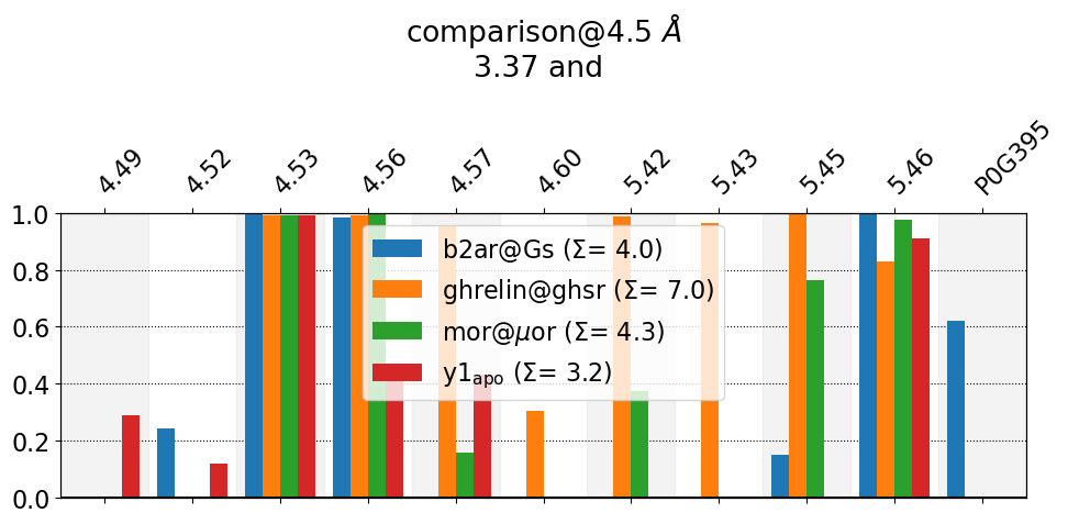
As we saw in the interface plot, 3.37 in ghrelin@ghsr has many more contacts than the other systems. Now we see why: that the Ghrelin-receptor’s 3.37 residue is interacting with TM4 and TM5 more than the rest.
Compare Contact-Distances
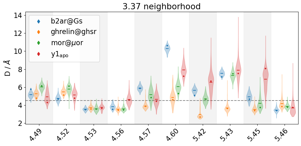
We will inspect this further, first using violin plots in the next cell:
[14]:
fig, ax, plotted_labels = mdciao.plots.compare_violins(rn337,
ctc_cutoff_Ang=4.5, defrag=None,
AA_format="try_consensus",
sort_by="consensus",
anchor="3.37",
figsize=None);
Turns out, 4.57, 4.60, 5.42, and 5.43 weren’t even included other 3.37 neighborhoods (mor@muor, b2ar@Gs, y1_apo), because they never came in contact with 3.37 (or almost never, according to min_freq=0.1, the default value of mdciao.cli.interface).
Still, we can use mdciao’s mdciao.cli.sites to provide an explict list of pairs of residues we want to look at, regardless of them forming a contact or not.
Sites
You guessed right, we can specifiy them simply using the consensus labels. We stored them in the cell above in the plotted_labels variable, so it’s very easy to pass them on to the site definitions:
[15]:
site_337_def = {"name": "selected 3.77 distances",
"pairs" : {"consensus" : [f"3.37-{label}" for label in plotted_labels]}}
site_337_def
[15]:
{'name': 'selected 3.77 distances',
'pairs': {'consensus': ['3.37-4.49',
'3.37-4.52',
'3.37-4.53',
'3.37-4.56',
'3.37-4.57',
'3.37-4.60',
'3.37-5.42',
'3.37-5.43',
'3.37-5.45',
'3.37-5.46',
'3.37-P0G395']}}
Again, feel free to comment in %%capture to see all outputs, but we will be comparing the distances two cells below anyways.
[16]:
%%capture
site_337 = {}
for system in systems:
site_337[system] = mdciao.cli.sites(site_337_def,
f"{system}/traj.xtc", topology=f"{system}/top.pdb", output_dir=system,
GPCR_UniProt=GPCR[system], accept_guess=True,
no_disk=True,allow_partial_sites=True,
CGN_UniProt=CGN.get(system, None),figures=False,
fragments="chains")["selected 3.77 distances"]
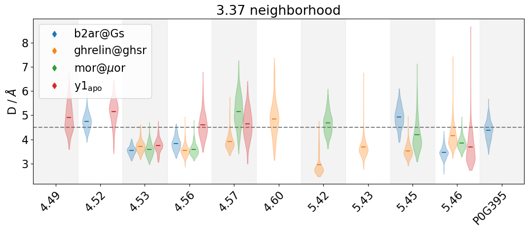
[17]:
fig, ax, plotted_labels, repframes = mdciao.plots.compare_violins(site_337, defrag=None,
AA_format="try_consensus",
anchor="3.37",
sort_by="consensus",
representatives=True,
ctc_cutoff_Ang=4.5,
);
Returning frame 149 of traj nr. 0: b2ar@Gs/traj.xtc
Returning frame 302 of traj nr. 0: ghrelin@ghsr/traj.xtc
Returning frame 35 of traj nr. 0: mor@muor/traj.xtc
Returning frame 331 of traj nr. 0: y1_apo/traj.xtc
We see that the distances for4.60, and 5.43 for mor@muor, b2ar@Gs, y1_apo virtually never cross the 4.5 Å cutoff.
Also note that by using representatives=True we have triggered some things in the violin plots. For each system, we have tried to locate a frame in the trajectory in which the shown residue-residue distances adopt values close to the most likely value (=where the violin is widest). You can read about these representative frames here:
ContactGroup.repframes.
These frames are represented as dots inside the individual violins and also as returned geometries in form of mdtraj trajectories (stored in the repframes returned value) which we can visualize in 3D.
Visualizing Representative Frames
The first thing we note is that geometries won’t be aligned, because they’re all coming from different simulations. Also, b2ar@Gs has the whole G-protein as well.
[18]:
import nglview
from matplotlib import colors as mplcolors
colors = mdciao.plots.color_dict_guesser("tab10", repframes.keys())
iwd = nglview.NGLWidget()
for ii, (system, geom) in enumerate(repframes.items()):
iwd.add_trajectory(geom)#, [[gpcr_idxs]]), title="test")
iwd.clear_representations(component=ii)
iwd.add_cartoon(component=ii, color=mplcolors.to_hex(colors[system]), name=system, radius=.1)
iwd
To produce a high quality alignment of the receptor structures, even with low primary-sequence identity, we can arrive at a multiple-sequence-alignment (MSA) via the consensus labels, which act as a proxy for sequence identity. For this, we use mdciao’s AlignerConsensus class. There’s a whole notebook about them
here.
[19]:
AC = mdciao.nomenclature.AlignerConsensus(GPCR, tops={key : val.top for key, val in repframes.items()})
Fragments derived from 'resSeq':
fragment 0 with 320 AAs PHE18 ( 0) - PHE337 (319 ) (0)
fragment 1 with 1 AAs ASP339 ( 320) - ASP339 (320 ) (1)
* Alignment 0
There are clashes between the above 'resSeq' definitions and the consensus fragments' definitions:
fragment C-term with 3 AAs ASN336 ( 318) - ASP339 (320 ) (C-term) resSeq jumps
clashes/spreads across these 'resSeq' fragments:
fragment 0 with 320 AAs PHE18 ( 0) - PHE337 (319 ) (0)
fragment 1 with 1 AAs ASP339 ( 320) - ASP339 (320 ) (1)
but all the residues of `top` that have been assigned to C-term using this alignment are contained
(= same name, same index) in the reference C-term, meaning, there's probably just a hole in C-term
in your `top`. Rerun with `verbose=True` to show that part of this alignment here.
=> C-term is hence considered compatible with alignment '0'.
Now that we have the AlignerConsensus object, we can use the sequence_match method to get an overview of how different the primary sequences are:
[20]:
AC.sequence_match()
[20]:
| b2ar@Gs | ghrelin@ghsr | mor@muor | y1_apo | |
|---|---|---|---|---|
| b2ar@Gs | 100% | 23% | 26% | 24% |
| ghrelin@ghsr | 23% | 100% | 26% | 24% |
| mor@muor | 26% | 26% | 100% | 26% |
| y1_apo | 24% | 24% | 26% | 100% |
We can do a lot of things with the AC object, e.g. this is the consensus-MSA for TM3
[21]:
AC.AAresSeq_match("3.*")
[21]:
| consensus | b2ar@Gs | ghrelin@ghsr | mor@muor | y1_apo | |
|---|---|---|---|---|---|
| 73 | 3.21 | G102 | G112 | G136 | G109 |
| 74 | 3.22 | N103 | D113 | N137 | E110 |
| 75 | 3.23 | F104 | L114 | I138 | A111 |
| 76 | 3.24 | W105 | L115 | L139 | M112 |
| 77 | 3.25 | C106 | C116 | C140 | C113 |
| 78 | 3.26 | E107 | K117 | K141 | K114 |
| 79 | 3.27 | F108 | L118 | I142 | L115 |
| 80 | 3.28 | W109 | F119 | V143 | N116 |
| 81 | 3.29 | T110 | Q120 | I144 | P117 |
| 82 | 3.30 | S111 | F121 | S145 | F118 |
| 83 | 3.31 | I112 | V122 | I146 | V119 |
| 84 | 3.32 | D113 | S123 | D147 | Q120 |
| 85 | 3.33 | V114 | E124 | Y148 | C121 |
| 86 | 3.34 | L115 | S125 | Y149 | V122 |
| 87 | 3.35 | C116 | C126 | N150 | S123 |
| 88 | 3.36 | V117 | T127 | M151 | I124 |
| 89 | 3.37 | T118 | Y128 | F152 | T125 |
| 90 | 3.38 | A119 | A129 | T153 | V126 |
| 91 | 3.39 | S120 | T130 | S154 | S127 |
| 92 | 3.40 | I121 | V131 | I155 | I128 |
| 93 | 3.41 | E122 | L132 | F156 | F129 |
| 94 | 3.42 | T123 | T133 | T157 | S130 |
| 95 | 3.43 | L124 | I134 | L158 | L131 |
| 96 | 3.44 | C125 | T135 | C159 | V132 |
| 97 | 3.45 | V126 | A136 | T160 | L133 |
| 98 | 3.46 | I127 | L137 | M161 | I134 |
| 99 | 3.47 | A128 | S138 | S162 | A135 |
| 100 | 3.48 | V129 | V139 | V163 | V136 |
| 101 | 3.49 | D130 | E140 | D164 | E137 |
| 102 | 3.50 | R131 | R141 | R165 | R138 |
| 103 | 3.51 | Y132 | Y142 | Y166 | H139 |
| 104 | 3.52 | F133 | F143 | I167 | Q140 |
| 105 | 3.53 | A134 | A144 | A168 | L141 |
| 106 | 3.54 | I135 | I145 | V169 | I142 |
| 107 | 3.55 | T136 | C146 | C170 | I143 |
| 108 | 3.56 | S137 | F147 | H171 | N144 |
Superpose Geometries
For the alignment we use the selection “?.*,-6.*,8.*” which selects all TMs, except TM6 and H8:
[22]:
CA_idxs = AC.CAidxs_match("?.*,-6.*,8.*")
[23]:
ref_key = "b2ar@Gs"
for ii, (system, geom) in enumerate(repframes.items()):
if system!=ref_key:
geom.superpose(repframes[ref_key], atom_indices=CA_idxs[system], ref_atom_indices=CA_idxs[ref_key])
Show Geometries
[24]:
iwd = nglview.NGLWidget()
for ii, (system, geom) in enumerate(repframes.items()):
iwd.add_trajectory(geom)
iwd.clear_representations(component=ii)
iwd.add_cartoon(component=ii, color=mplcolors.to_hex(colors[system]), name=system, radius=.1)
iwd
Show 3.37’s neighborhood
Finally, we fine-tune the 3D representation to include the most varying contacts of 3.37: 4.60, 5.42, and 5.43, which we show first as a table across the four systems:
[25]:
show=["3.37","4.60", "5.42", "5.43"]
AC.AAresSeq_match(",".join(show))
[25]:
| consensus | b2ar@Gs | ghrelin@ghsr | mor@muor | y1_apo | |
|---|---|---|---|---|---|
| 89 | 3.37 | T118 | Y128 | F152 | T125 |
| 139 | 4.60 | P168 | I178 | V202 | F173 |
| 159 | 5.42 | S203 | V216 | V236 | L215 |
| 160 | 5.43 | S204 | S217 | F237 | L216 |
[26]:
iwd = nglview.NGLWidget()
ref_key = "b2ar@Gs"
for ii, (system, geom) in enumerate(repframes.items()):
iwd.add_trajectory(geom, title=system)
iwd.clear_representations(component=ii)
iwd.add_cartoon(component=ii, color=mplcolors.to_hex(colors[system]), name=system, radius=.1)
AAs = " ".join([GPCR[system].conlab2AA[jj][1:] for jj in show])
iwd.add_licorice(component=ii, selection=f"({AAs}) and not Hydrogen", radius=.5, color=mplcolors.to_hex(colors[system]))
iwd.gui_style = "ngl"
iwd
From the 3D plot above we can make some observations, most clearly we note that ghrelin@ghsr has the bulikest residue, Y128@3.50, which is pointing straight down to a region where TM5 appears to have a bulge, precisely towards the 3.50 position, something the other TM5s don’t have.
Final Remarks
Some final observations
The point of this notebook isn’t to arrive at a particular finding but rather to showcase the utility of streamilining the contact-analysis across diffeent systems using consensus nomenclature.
We have kept the system names as they are downloaded with mdciao.examples.fetch_example_data, because they all follow the convention of having a
traj.xtcandtop.pdbfiles, but you can map any topology and trajectory files using aliases and dictionaries:alias = {"b2ar@Gs" : "adrb2", "ghrelin@ghsr" : "ghsr", "mor@muor" : "muor", "y1_apo" : "y1" } #these are just examples of possible other topology filenames. top = {"adrb2" : "adrb2/prot1.pdb", "ghsr" : "ghrelin/system.pdb", "muor" : "muor/muor.pdb", "y1" : "y1/top.pdb" } #these are just examples of possible other trajectory filenames. trajs = {"adrb2" : "adrb2/traj.xtc", "ghsr" : "ghrelin/traj1.xtc", "ghrelin/traj2.xtc", "muor" : "muor/run*.xtc", "y1" : "y1/run1.xtc" }
Althouth the trajectories we have been using are similar in number of frames, they are wildly different in simulated physical length, s.o there isn’t really much physical or biological sense in comparing them other than for this demo:
* b2ar@Gs: 280 frames, dt = 10ps, 2.8ns in total
* ghrelin@ghsr: 411 frames, dt = 10ns, 41μs in total
* mor@muor: 400 frames, dt = 10ns, 40μs in total
* y1_apo: 528 frames, dt = 50ns, 26.4ns in total
[ ]: