Interface of β2 Adrenergic Receptor in Complex with Empty Gs-Protein
[1]:
import mdtraj as md
import mdciao
Download example data and load into the namespace
[2]:
import numpy as np
import os
if not os.path.exists("mdciao_example"):
    mdciao.examples.fetch_example_data("b2ar@Gs")
traj = md.load("mdciao_example/traj.xtc",top="mdciao_example/top.pdb")
Create consensus labeler objects
[3]:
GPCR = mdciao.nomenclature.LabelerGPCR("adrb2_human")
CGN = mdciao.nomenclature.LabelerCGN("GNAS2_HUMAN")
No local file ./adrb2_human.xlsx found, checking online in
https://gpcrdb.org/services/residues/extended/adrb2_human ...done!
Please cite the following reference to the GPCRdb:
 * Kooistra et al, (2021) GPCRdb in 2021: Integrating GPCR sequence, structure and function
   Nucleic Acids Research 49, D335--D343
   https://doi.org/10.1093/nar/gkaa1080
For more information, call mdciao.nomenclature.references()
No local file ./GNAS2_HUMAN.xlsx found, checking online in
https://gpcrdb.org/services/residues/extended/gnas2_human ...done!
Please cite the following reference to the GPCRdb:
 * Kooistra et al, (2021) GPCRdb in 2021: Integrating GPCR sequence, structure and function
   Nucleic Acids Research 49, D335--D343
   https://doi.org/10.1093/nar/gkaa1080
Please cite the following reference to the CGN nomenclature:
 * Flock et al, (2015) Universal allosteric mechanism for G$\alpha$ activation by GPCRs
   Nature 2015 524:7564 524, 173--179
   https://doi.org/10.1038/nature14663
For more information, call mdciao.nomenclature.references()
Guess molecular fragments
This would be done anyway by the mdciao.cli.interface call in the cell below, here we do it have the fragments defined in the namespace
[4]:
fragments = mdciao.fragments.get_fragments(traj.top);
fragment_names = ["Galpha", "Gbeta", "Ggamma","B2AR","P0G"]
Auto-detected fragments with method 'lig_resSeq+'
fragment      0 with    354 AAs     LEU4 (   0) -   LEU394 (353 ) (0) resSeq jumps
fragment      1 with    340 AAs     GLN1 ( 354) -   ASN340 (693 ) (1)
fragment      2 with     66 AAs     ALA2 ( 694) -    PHE67 (759 ) (2)
fragment      3 with    283 AAs    GLU30 ( 760) -   LEU340 (1042) (3) resSeq jumps
fragment      4 with      1 AAs   P0G395 (1043) -   P0G395 (1043) (4)
Compute G\(\alpha\)-B2AR interface
Using the above fragment definitions
[5]:
intf = mdciao.cli.interface(traj,
                            title="3SN6 beta2AR-Galpha interface",
                            fragments=fragments, fragment_names = fragment_names,
                            interface_selection_1=[0],
                            interface_selection_2=[3],
                            GPCR_UniProt=GPCR, CGN_UniProt=CGN,
                            accept_guess=True, no_disk=True, figures=False)
Will compute contact frequencies for trajectories:
<mdtraj.Trajectory with 280 frames, 8384 atoms, 1044 residues, and unitcells>
 with a stride of 1 frames
Using method 'user input by residue array or range' these fragments were found
fragment Galpha with    354 AAs     LEU4 (   0) -   LEU394 (353 ) (Galpha) resSeq jumps
fragment Gbeta  with    340 AAs     GLN1 ( 354) -   ASN340 (693 ) (Gbeta)
fragment Ggamma with     66 AAs     ALA2 ( 694) -    PHE67 (759 ) (Ggamma)
fragment B2AR   with    283 AAs    GLU30 ( 760) -   LEU340 (1042) (B2AR) resSeq jumps
fragment P0G    with      1 AAs   P0G395 (1043) -   P0G395 (1043) (P0G)
The GPCR-labels align best with fragments: [3] (first-last: GLU30-LEU340).

Mapping the GPCR fragments onto your topology:
 TM1  with     32 AAs    GLU30@1.29x29   ( 760) -    PHE61@1.60x60   (791 ) (TM1)
 ICL1 with      4 AAs    GLU62@12.48x48  ( 792) -    GLN65@12.51x51  (795 ) (ICL1)
 TM2  with     32 AAs    THR66@2.37x37   ( 796) -    LYS97@2.68x67   (827 ) (TM2)
 ECL1 with      4 AAs    MET98@23.49x49  ( 828) -   PHE101@23.52x52  (831 ) (ECL1)
 TM3  with     36 AAs   GLY102@3.21x21   ( 832) -   SER137@3.56x56   (867 ) (TM3)
 ICL2 with      8 AAs   PRO138@34.50x50  ( 868) -   LEU145@34.57x57  (875 ) (ICL2)
 TM4  with     27 AAs   THR146@4.38x38   ( 876) -   HIS172@4.64x64   (902 ) (TM4)
 ECL2 with     20 AAs   TRP173           ( 903) -   THR195           (922 ) (ECL2) resSeq jumps
 TM5  with     42 AAs   ASN196@5.35x36   ( 923) -   GLU237@5.76x76   (964 ) (TM5)
 ICL3 with      2 AAs   GLY238           ( 965) -   ARG239           (966 ) (ICL3)
 TM6  with     35 AAs   CYS265@6.27x27   ( 967) -   GLN299@6.61x61   (1001) (TM6)
 ECL3 with      4 AAs   ASP300           (1002) -   ILE303           (1005) (ECL3)
 TM7  with     25 AAs   ARG304@7.31x30   (1006) -   ARG328@7.55x55   (1030) (TM7)
 H8   with     12 AAs   SER329@8.47x47   (1031) -   LEU340@8.58x58   (1042) (H8)
The CGN-labels align best with fragments: [0] (first-last: LEU4-LEU394).

Mapping the CGN fragments onto your topology:
 G.HN   with     33 AAs     LEU4@G.HN.10   (   0) -    VAL36@G.HN.53   (32  ) (G.HN)
 G.hns1 with      3 AAs    TYR37@G.hns1.01 (  33) -    ALA39@G.hns1.03 (35  ) (G.hns1)
 G.S1   with      7 AAs    THR40@G.S1.01   (  36) -    LEU46@G.S1.07   (42  ) (G.S1)
 G.s1h1 with      6 AAs    GLY47@G.s1h1.01 (  43) -    GLY52@G.s1h1.06 (48  ) (G.s1h1)
 G.H1   with      7 AAs    LYS53@G.H1.01   (  49) -    GLN59@G.H1.07   (55  ) (G.H1)
 H.HA   with     26 AAs    LYS88@H.HA.04   (  56) -   LEU113@H.HA.29   (81  ) (H.HA)
 H.hahb with      9 AAs   VAL114@H.hahb.01 (  82) -   PRO122@H.hahb.09 (90  ) (H.hahb)
 H.HB   with     14 AAs   GLU123@H.HB.01   (  91) -   ASN136@H.HB.14   (104 ) (H.HB)
 H.hbhc with      7 AAs   VAL137@H.hbhc.01 ( 105) -   PRO143@H.hbhc.15 (111 ) (H.hbhc)
 H.HC   with     12 AAs   PRO144@H.HC.01   ( 112) -   GLU155@H.HC.12   (123 ) (H.HC)
 H.hchd with      1 AAs   ASP156@H.hchd.01 ( 124) -   ASP156@H.hchd.01 (124 ) (H.hchd)
 H.HD   with     12 AAs   GLU157@H.HD.01   ( 125) -   GLU168@H.HD.12   (136 ) (H.HD)
 H.hdhe with      5 AAs   TYR169@H.hdhe.01 ( 137) -   ASP173@H.hdhe.05 (141 ) (H.hdhe)
 H.HE   with     13 AAs   CYS174@H.HE.01   ( 142) -   LYS186@H.HE.13   (154 ) (H.HE)
 H.hehf with      7 AAs   GLN187@H.hehf.01 ( 155) -   SER193@H.hehf.07 (161 ) (H.hehf)
 H.HF   with      6 AAs   ASP194@H.HF.01   ( 162) -   ARG199@H.HF.06   (167 ) (H.HF)
 G.hfs2 with      5 AAs   CYS200@G.hfs2.01 ( 168) -   GLY206@G.hfs2.07 (172 ) (G.hfs2) resSeq jumps
 G.S2   with      8 AAs   ILE207@G.S2.01   ( 173) -   VAL214@G.S2.08   (180 ) (G.S2)
 G.s2s3 with      2 AAs   ASP215@G.s2s3.01 ( 181) -   LYS216@G.s2s3.02 (182 ) (G.s2s3)
 G.S3   with      8 AAs   VAL217@G.S3.01   ( 183) -   VAL224@G.S3.08   (190 ) (G.S3)
 G.s3h2 with      3 AAs   GLY225@G.s3h2.01 ( 191) -   GLN227@G.s3h2.03 (193 ) (G.s3h2)
 G.H2   with     10 AAs   ARG228@G.H2.01   ( 194) -   CYS237@G.H2.10   (203 ) (G.H2)
 G.h2s4 with      5 AAs   PHE238@G.h2s4.01 ( 204) -   THR242@G.h2s4.05 (208 ) (G.h2s4)
 G.S4   with      7 AAs   ALA243@G.S4.01   ( 209) -   ALA249@G.S4.07   (215 ) (G.S4)
 G.s4h3 with      8 AAs   SER250@G.s4h3.01 ( 216) -   ASN264@G.s4h3.15 (223 ) (G.s4h3) resSeq jumps
 G.H3   with     18 AAs   ARG265@G.H3.01   ( 224) -   LEU282@G.H3.18   (241 ) (G.H3)
 G.h3s5 with      3 AAs   ARG283@G.h3s5.01 ( 242) -   ILE285@G.h3s5.03 (244 ) (G.h3s5)
 G.S5   with      7 AAs   SER286@G.S5.01   ( 245) -   ASN292@G.S5.07   (251 ) (G.S5)
 G.s5hg with      1 AAs   LYS293@G.s5hg.01 ( 252) -   LYS293@G.s5hg.01 (252 ) (G.s5hg)
 G.HG   with     17 AAs   GLN294@G.HG.01   ( 253) -   ASP310@G.HG.17   (269 ) (G.HG)
 G.hgh4 with     21 AAs   TYR311@G.hgh4.01 ( 270) -   ASP331@G.hgh4.21 (290 ) (G.hgh4)
 G.H4   with     16 AAs   PRO332@G.H4.01   ( 291) -   ARG347@G.H4.17   (306 ) (G.H4)
 G.h4s6 with     11 AAs   ILE348@G.h4s6.01 ( 307) -   TYR358@G.h4s6.20 (317 ) (G.h4s6)
 G.S6   with      5 AAs   CYS359@G.S6.01   ( 318) -   PHE363@G.S6.05   (322 ) (G.S6)
 G.s6h5 with      5 AAs   THR364@G.s6h5.01 ( 323) -   ASP368@G.s6h5.05 (327 ) (G.s6h5)
 G.H5   with     26 AAs   THR369@G.H5.01   ( 328) -   LEU394@G.H5.26   (353 ) (G.H5)
Select group 1: 0
Select group 2: 3

Will look for contacts in the interface between fragments
0
and
3.

Performing a first pass on the 100182 group_1-group_2 residue pairs to compute lower bounds on residue-residue distances via residue-COM distances.
Reduced to only 912 (from 100182) residue pairs for the computation of actual residue-residue distances:
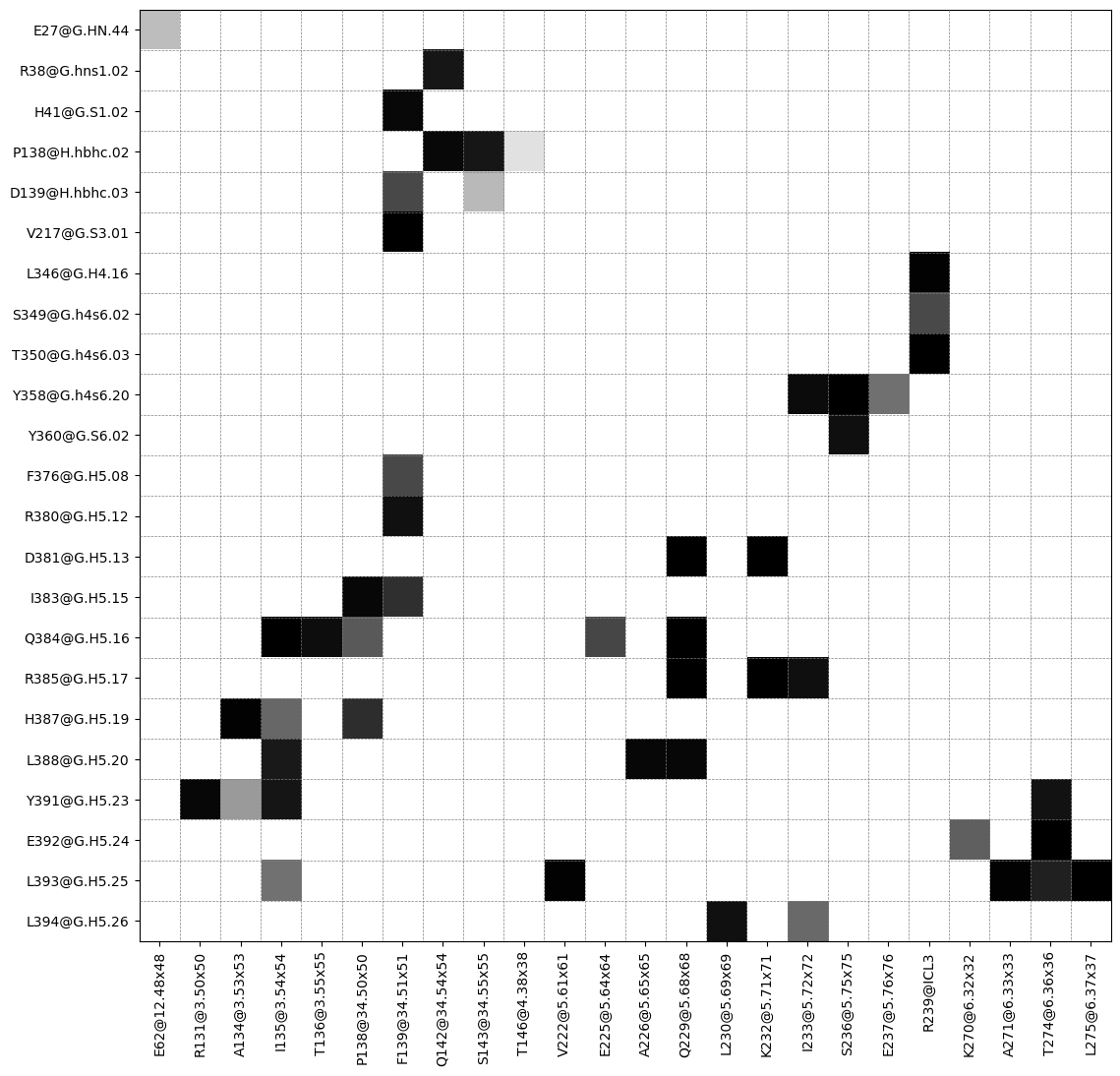
The following 50 contacts capture 45.66 (~91%) of the total frequency 50.28 (over 107 contacts with nonzero frequency at 4.50 Angstrom).
As orientation value, the first 50 ctcs already capture 90.0% of 50.28.
The 50-th contact has a frequency of 0.52.
freq label residues fragments sum
1 1.00 R385@G.H5.17 - K232@5.71x71 344 - 959 0 - 3 1.00
2 1.00 V217@G.S3.01 - F139@34.51x51 183 - 869 0 - 3 2.00
3 1.00 R385@G.H5.17 - Q229@5.68x68 344 - 956 0 - 3 3.00
4 1.00 D381@G.H5.13 - Q229@5.68x68 340 - 956 0 - 3 4.00
5 1.00 E392@G.H5.24 - T274@6.36x36 351 - 976 0 - 3 5.00
6 1.00 Y358@G.h4s6.20 - S236@5.75x75 317 - 963 0 - 3 6.00
7 1.00 D381@G.H5.13 - K232@5.71x71 340 - 959 0 - 3 7.00
8 1.00 Q384@G.H5.16 - I135@3.54x54 343 - 865 0 - 3 8.00
9 1.00 T350@G.h4s6.03 - R239@ICL3 309 - 966 0 - 3 9.00
10 1.00 L393@G.H5.25 - L275@6.37x37 352 - 977 0 - 3 9.99
11 1.00 Q384@G.H5.16 - Q229@5.68x68 343 - 956 0 - 3 10.99
12 0.99 H387@G.H5.19 - A134@3.53x53 346 - 864 0 - 3 11.98
13 0.99 L393@G.H5.25 - V222@5.61x61 352 - 949 0 - 3 12.98
14 0.99 L393@G.H5.25 - A271@6.33x33 352 - 973 0 - 3 13.97
15 0.99 L346@G.H4.16 - R239@ICL3 305 - 966 0 - 3 14.96
16 0.99 Y391@G.H5.23 - R131@3.50x50 350 - 861 0 - 3 15.95
17 0.99 L388@G.H5.20 - A226@5.65x65 347 - 953 0 - 3 16.93
18 0.99 L388@G.H5.20 - Q229@5.68x68 347 - 956 0 - 3 17.92
19 0.99 I383@G.H5.15 - P138@34.50x50 342 - 868 0 - 3 18.90
20 0.98 P138@H.hbhc.02 - Q142@34.54x54 106 - 872 0 - 3 19.89
21 0.98 H41@G.S1.02 - F139@34.51x51 37 - 869 0 - 3 20.87
22 0.98 Y358@G.h4s6.20 - I233@5.72x72 317 - 960 0 - 3 21.85
23 0.98 Q384@G.H5.16 - T136@3.55x55 343 - 866 0 - 3 22.82
24 0.97 Y360@G.S6.02 - S236@5.75x75 319 - 963 0 - 3 23.79
25 0.97 R385@G.H5.17 - I233@5.72x72 344 - 960 0 - 3 24.76
26 0.97 L394@G.H5.26 - L230@5.69x69 353 - 957 0 - 3 25.73
27 0.97 R380@G.H5.12 - F139@34.51x51 339 - 869 0 - 3 26.70
28 0.96 Y391@G.H5.23 - T274@6.36x36 350 - 976 0 - 3 27.66
29 0.96 Y391@G.H5.23 - I135@3.54x54 350 - 865 0 - 3 28.63
30 0.96 P138@H.hbhc.02 - S143@34.55x55 106 - 873 0 - 3 29.58
31 0.96 R38@G.hns1.02 - Q142@34.54x54 34 - 872 0 - 3 30.54
32 0.95 L388@G.H5.20 - I135@3.54x54 347 - 865 0 - 3 31.49
33 0.94 L393@G.H5.25 - T274@6.36x36 352 - 976 0 - 3 32.43
34 0.91 H387@G.H5.19 - P138@34.50x50 346 - 868 0 - 3 33.34
35 0.91 I383@G.H5.15 - F139@34.51x51 342 - 869 0 - 3 34.25
36 0.87 Q384@G.H5.16 - E225@5.64x64 343 - 952 0 - 3 35.12
37 0.86 F376@G.H5.08 - F139@34.51x51 335 - 869 0 - 3 35.99
38 0.86 D139@H.hbhc.03 - F139@34.51x51 107 - 869 0 - 3 36.85
39 0.86 S349@G.h4s6.02 - R239@ICL3 308 - 966 0 - 3 37.71
40 0.83 Q384@G.H5.16 - P138@34.50x50 343 - 868 0 - 3 38.54
41 0.82 E392@G.H5.24 - K270@6.32x32 351 - 972 0 - 3 39.36
42 0.81 H387@G.H5.19 - I135@3.54x54 346 - 865 0 - 3 40.17
43 0.80 L394@G.H5.26 - I233@5.72x72 353 - 960 0 - 3 40.97
44 0.79 Y358@G.h4s6.20 - E237@5.76x76 317 - 964 0 - 3 41.76
45 0.79 L393@G.H5.25 - I135@3.54x54 352 - 865 0 - 3 42.55
46 0.71 Y391@G.H5.23 - A134@3.53x53 350 - 864 0 - 3 43.26
47 0.65 D139@H.hbhc.03 - S143@34.55x55 107 - 873 0 - 3 43.91
48 0.65 E27@G.HN.44 - E62@12.48x48 23 - 792 0 - 3 44.56
49 0.58 P138@H.hbhc.02 - T146@4.38x38 106 - 876 0 - 3 45.14
50 0.52 L394@G.H5.26 - K270@6.32x32 353 - 972 0 - 3 45.66
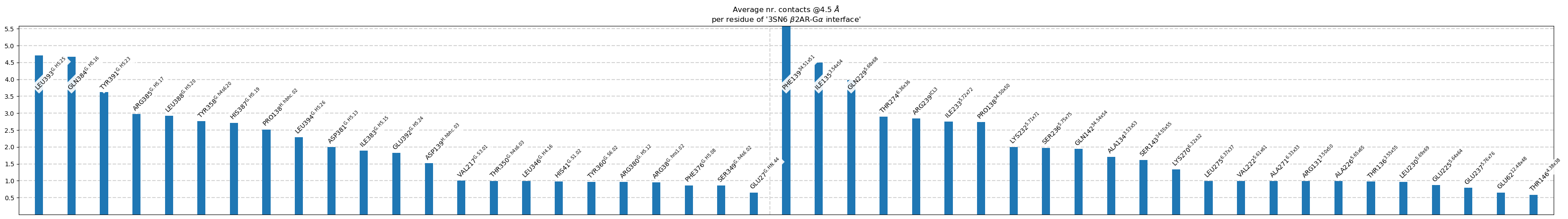
label freq
1 L393@G.H5.25 4.71
2 Q384@G.H5.16 4.67
3 Y391@G.H5.23 3.62
4 R385@G.H5.17 2.97
5 L388@G.H5.20 2.92
6 Y358@G.h4s6.20 2.77
7 H387@G.H5.19 2.71
8 P138@H.hbhc.02 2.52
9 L394@G.H5.26 2.29
10 D381@G.H5.13 2.00
11 I383@G.H5.15 1.90
12 E392@G.H5.24 1.82
13 D139@H.hbhc.03 1.52
14 V217@G.S3.01 1.00
15 T350@G.h4s6.03 1.00
16 L346@G.H4.16 0.99
17 H41@G.S1.02 0.98
18 Y360@G.S6.02 0.97
19 R380@G.H5.12 0.97
20 R38@G.hns1.02 0.96
21 F376@G.H5.08 0.86
22 S349@G.h4s6.02 0.86
23 E27@G.HN.44 0.65
label freq
1 F139@34.51x51 5.59
2 I135@3.54x54 4.50
3 Q229@5.68x68 3.98
4 T274@6.36x36 2.90
5 R239@ICL3 2.85
6 I233@5.72x72 2.75
7 P138@34.50x50 2.73
8 K232@5.71x71 2.00
9 S236@5.75x75 1.97
10 Q142@34.54x54 1.94
11 A134@3.53x53 1.70
12 S143@34.55x55 1.61
13 K270@6.32x32 1.34
14 L275@6.37x37 1.00
15 V222@5.61x61 0.99
16 A271@6.33x33 0.99
17 R131@3.50x50 0.99
18 A226@5.65x65 0.99
19 T136@3.55x55 0.98
20 L230@5.69x69 0.97
21 E225@5.64x64 0.87
22 E237@5.76x76 0.79
23 E62@12.48x48 0.65
24 T146@4.38x38 0.58
Plot each residues’s participation in the interface
[6]:
ifig = intf.plot_frequency_sums_as_bars(4.5, title_str = intf.name,
                                 list_by_interface=True,
                                 interface_vline=True);
ifig.figure.savefig("intf.svg")
Plot contact matrix
[7]:
ifig, iax = intf.plot_interface_frequency_matrix(4.5, grid=True, pixelsize=.5);
ifig.savefig("matrix.svg")
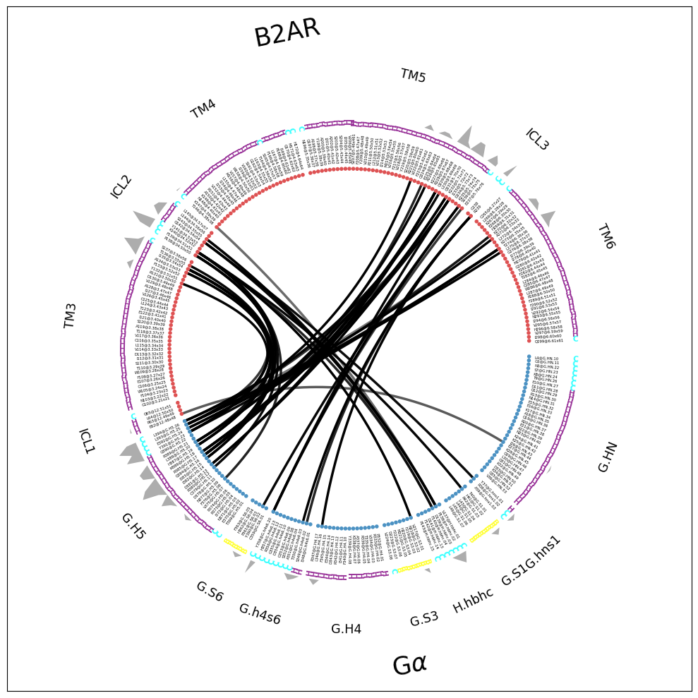
Flareplot
We combine a lot of information into one single flareplot:
the molecular topology with sub-fragments and consensus labels,
the secondary structure,
the individual contact-pairs
the participation of each residue in the interface.
[8]:
ifig, iax, flareplot_attrs  = intf.plot_freqs_as_flareplot(4.5,
                                                           fragments=fragments, fragment_names = fragment_names,
                                                           scheme="consensus_sparse", consensus_maps=[GPCR, CGN],
                                                           aura=intf.frequency_sum_per_residue_idx_dict(4,return_array=True),
                                                           SS=True)
ifig.figure.savefig("flare.svg")
Drawing this many dots (270 residues + 18 padding spaces) in a panel 10.0 inches wide/high
forces too small dotsizes and fontsizes. If crowding effects occur, either reduce the
number of residues or increase the panel size
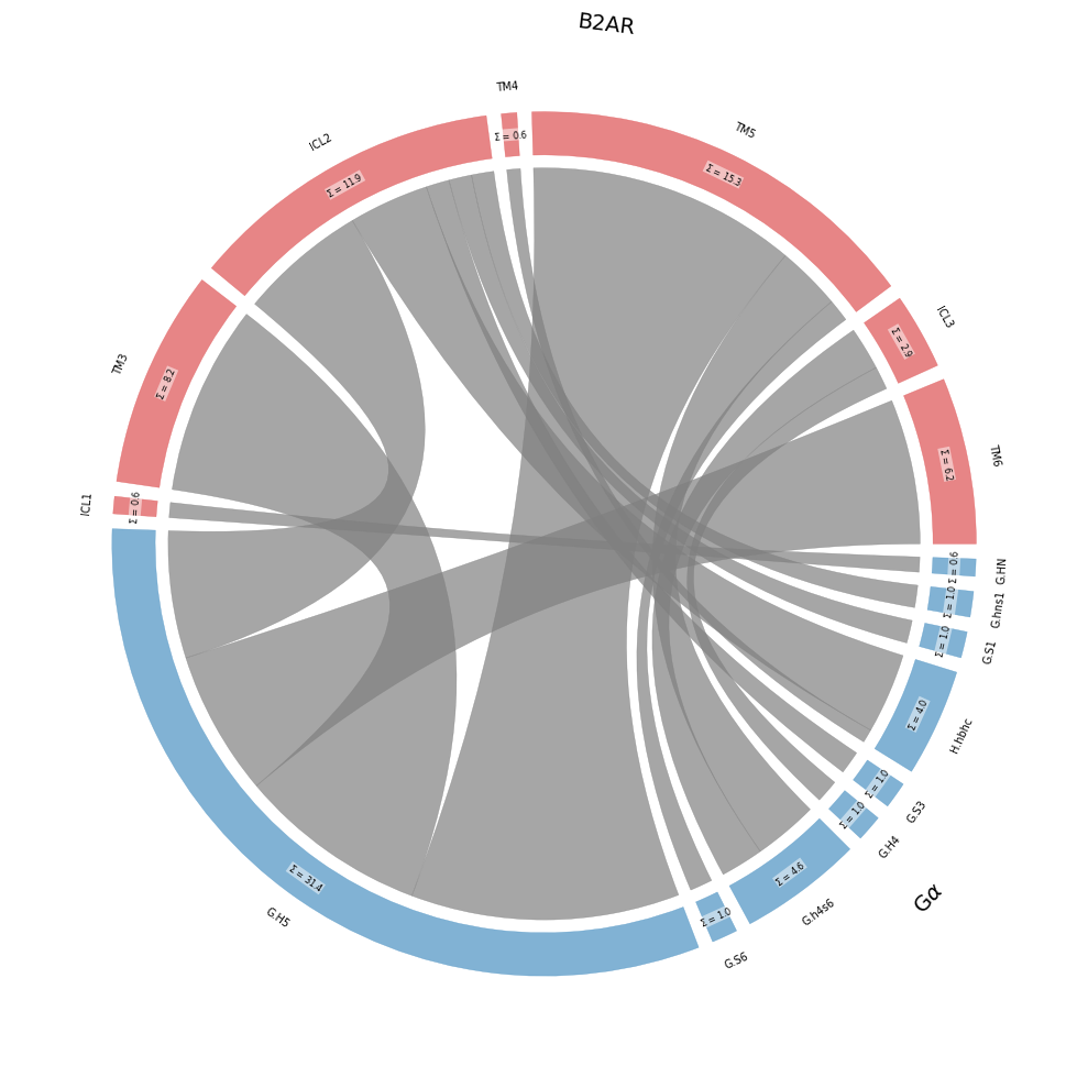
Coarse-Grained Frequencies and Flareplots
[9]:
ifig, iax, flareplot_attrs = intf.plot_freqs_as_flareplot(4.5,
                                                          fragments=fragments, fragment_names = fragment_names,
                                                          consensus_maps=[GPCR, CGN],
                                                          coarse_grain=True,
                                                         )
ifig.savefig("chord.svg",bbox_inches="tight")
freqs = intf.frequency_as_contact_matrix_CG(4.5, fragments=fragments, fragment_names = fragment_names,
                                            consensus_labelers=[GPCR, CGN],
                                            interface=True).round(1).replace(0,"")
freqs
[9]:
| ICL1 | TM3 | ICL2 | TM4 | TM5 | ICL3 | TM6 | |
|---|---|---|---|---|---|---|---|
| G.HN | 0.6 | ||||||
| G.hns1 | 1.0 | ||||||
| G.S1 | 1.0 | ||||||
| H.hbhc | 3.5 | 0.6 | |||||
| G.S3 | 1.0 | ||||||
| G.H4 | 1.0 | ||||||
| G.h4s6 | 2.8 | 1.9 | |||||
| G.S6 | 1.0 | ||||||
| G.H5 | 8.2 | 5.5 | 11.6 | 6.2 |
Grab a representative frame
This frame will be used to plot the interface frequencies as a 3D heatmap (see frequency_to_bfactor below).
[10]:
repframe = intf.repframes(return_traj=True)[-1]
Returning frame 202 of traj nr. 0: <mdtraj.Trajectory with 280 frames, 8384 atoms, 1044 residues, and unitcells>
Save the interface as a heatmap and view externally
[11]:
intf.frequency_to_bfactor(4.5, pdbfile="interface_heatmap.pdb",
                          geom=repframe,
                          interface_sign=True
                         );
Contact frequencies stored as signed bfactor in 'interface_heatmap.pdb'
Save all mdciao objects for later reuse
We can save all mdciao objects to numpy .npy (pickle) files and later reload them without having to compute everything again.
[12]:
import numpy as np
np.save("GPCR.npy", GPCR)
np.save("CGN.npy",CGN)
np.save("intf.npy",intf)