Missing Contacts
You might find that some contacts that you were expecting to be found by mdciao don’t actually show up in mdciao’s results. Several input parameters control the contact reporting of mdciao, and it might not be obvious which one of them (if any) is actually hiding your contact. The logic behind these parameters, and their default values, is fairly straightforward, and we illustrate it here.
If you want to run this notebook on your own, please download and extract the data from here first. You can download it:
using the browser
using the terminal with
wget http://proteinformatics.org/mdciao/mdciao_example.zip; unzip mdciao_example.zipusing mdciao’s own method mdciao.examples.fetch_example_data
If you want to take a 3D-look at this data, you can do it here.
ctc_cutoff_Ang
This is the most obvious parameter that controls the contact computation. It appears virtually in all methods (CLI or API) that compute contact frequencies. Whenever it has a default value, it is 4.5 Angstrom.
Note
Please see the note of caution on the use of hard cutoffs in the main page of the docs.
[1]:
import mdciao, os
if not os.path.exists("mdciao_example"):
    mdciao.examples.fetch_example_data()
[2]:
import mdtraj as md
traj = md.load("mdciao_example/traj.xtc",top="mdciao_example/top.pdb")
First, we individually call mdciao.cli.residue_neighborhoods with two ctc_cutoff_Ang values, 3.0, 3.5, and 4.0 Angstrom. This will generate three frequency reports which we will later compare with mdciao.cli.compare. Please refer to those methods if their function calls aren’t
entirely clear to you.
Note
We are hiding the outputs with the use of the `%%capture magic <https://ipython.readthedocs.io/en/stable/interactive/magics.html#cellmagic-capture>`__.
[3]:
%%capture
for ctc_cutoff_Ang in [3, 3.5, 4.0, 4.5, 5.0]:
    mdciao.cli.residue_neighborhoods("L394",traj,
                                     short_AA_names=True,
                                     ctc_cutoff_Ang=ctc_cutoff_Ang,
                                     figures=False,
                                     fragment_names=None,
                                     #ctc_control=1.0,
                                     no_disk=False)[353]
[4]:
mdciao.cli.compare({
    "ctc_cutoff_Ang = 5.0 AA" : "neighborhood.LEU394@5.0_Ang.dat",
    "ctc_cutoff_Ang = 4.5 AA" : "neighborhood.LEU394@4.5_Ang.dat",
    "ctc_cutoff_Ang = 4.0 AA" : "neighborhood.LEU394@4.0_Ang.dat",
    "ctc_cutoff_Ang = 3.5 AA" : "neighborhood.LEU394@3.5_Ang.dat",
    "ctc_cutoff_Ang = 3.0 AA" : "neighborhood.LEU394@3.0_Ang.dat",
                   },
                   anchor="L394",
                  title="Cutoff comparison");
These interactions are not shared:
I233, L230, R385
Their cumulative ctc freq is 8.00.
Created files
freq_comparison.pdf
freq_comparison.xlsx
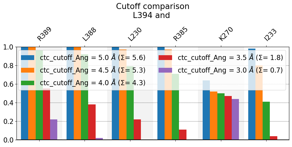
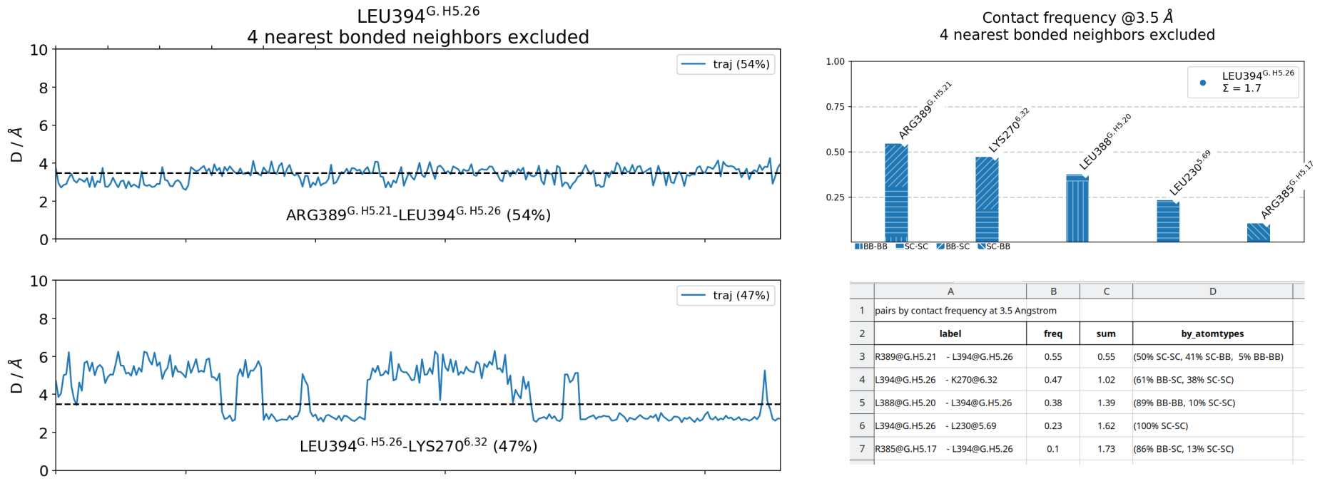
We observe that the smaller the cutoff, the fewer contacts get reported. In this case L230, R385, and I233 never approach L394 at distances smaller than 3.0 Angstrom during in the entire simulation, hence they don’t get reported (they don’t get any purple-bars). As for K270, the frequency doesn’t change very much, because it’s a salt-bridge that’s really either formed at very close distance or broken at higher distances, as can be seen in this time-trace
figure. Also notice that, the higher the cutoff, the higher the sum over bars, \(\Sigma\), since the height of the bars has increased.
ctc_control
Even when using the same ctc_cutoff_Ang, there’s other ways of controlling what gets reported. ctc_control is one of them. This parameter controls how many residues get reported per neighborhood, since usually one is not interested in all residues but only the most frequent ones.
Controlling with integers
One way to control this is to select only the first n frequent ones (n is an integer and is 6 by default). Here we do the comparison again, but withoug hiding the output s.t. you can see the contact list grow.
[5]:
#%%capture
ctc_controls = [4,5,6,7,8]
for ctc_control in ctc_controls:
    mdciao.cli.residue_neighborhoods("L394",traj,
                                     short_AA_names=True,
                                     ctc_control=ctc_control,
                                     figures=False,
                                     fragment_names=None,
                                     no_disk=False,
                                     output_desc='neighborhood.ctc_control_%u'%ctc_control)
mdciao.cli.compare({"ctc-control = %u"%key : "neighborhood.ctc_control_%u.LEU394@4.5_Ang.dat"%(key)
                   for key in ctc_controls},
                   anchor="L394",
                   title="ctc-control comparison");
Will compute contact frequencies for (1 items):
<mdtraj.Trajectory with 280 frames, 8384 atoms, 1044 residues, and unitcells>
 with a stride of 1 frames
Using method 'lig_resSeq+' these fragments were found
fragment 0 with    354 AAs     LEU4 (   0) -   LEU394 (353 ) (0) resSeq jumps
fragment 1 with    340 AAs     GLN1 ( 354) -   ASN340 (693 ) (1)
fragment 2 with     66 AAs     ALA2 ( 694) -    PHE67 (759 ) (2)
fragment 3 with    283 AAs    GLU30 ( 760) -   LEU340 (1042) (3) resSeq jumps
fragment 4 with      1 AAs   P0G395 (1043) -   P0G395 (1043) (4)

Will compute neighborhoods for the residues
L394
excluding 4 nearest neighbors

   residue      residx    fragment      resSeq
    LEU394         353           0         394

Performing a first pass on 1039 residue pairs to compute lower bounds on residue-residue distances via residue-COM distances:
Reduced to only 43 residue pairs for the computation of actual residue-residue distances:
L394:
The following 4 contacts capture 3.94 (~72%) of the total frequency 5.43 (over 9 contacts with nonzero frequency at 4.50 Angstrom).
As orientation value, the first 6 ctcs already capture 90.0% of 5.43.
The 6-th contact has a frequency of 0.52.
   freq    label      residues  fragments   sum
1  1.00  L394 - L388  353 - 347    0 - 0   1.00
2  1.00  L394 - R389  353 - 348    0 - 0   2.00
3  0.97  L394 - L230  353 - 957    0 - 3   2.97
4  0.97  L394 - R385  353 - 344    0 - 0   3.94
The following files have been created:
./neighborhood.ctc_control_4.LEU394@4.5_Ang.dat
Will compute contact frequencies for (1 items):
<mdtraj.Trajectory with 280 frames, 8384 atoms, 1044 residues, and unitcells>
 with a stride of 1 frames
Using method 'lig_resSeq+' these fragments were found
fragment 0 with    354 AAs     LEU4 (   0) -   LEU394 (353 ) (0) resSeq jumps
fragment 1 with    340 AAs     GLN1 ( 354) -   ASN340 (693 ) (1)
fragment 2 with     66 AAs     ALA2 ( 694) -    PHE67 (759 ) (2)
fragment 3 with    283 AAs    GLU30 ( 760) -   LEU340 (1042) (3) resSeq jumps
fragment 4 with      1 AAs   P0G395 (1043) -   P0G395 (1043) (4)

Will compute neighborhoods for the residues
L394
excluding 4 nearest neighbors

   residue      residx    fragment      resSeq
    LEU394         353           0         394

Performing a first pass on 1039 residue pairs to compute lower bounds on residue-residue distances via residue-COM distances:
Reduced to only 43 residue pairs for the computation of actual residue-residue distances:
L394:
The following 5 contacts capture 4.74 (~87%) of the total frequency 5.43 (over 9 contacts with nonzero frequency at 4.50 Angstrom).
As orientation value, the first 6 ctcs already capture 90.0% of 5.43.
The 6-th contact has a frequency of 0.52.
   freq    label      residues  fragments   sum
1  1.00  L394 - L388  353 - 347    0 - 0   1.00
2  1.00  L394 - R389  353 - 348    0 - 0   2.00
3  0.97  L394 - L230  353 - 957    0 - 3   2.97
4  0.97  L394 - R385  353 - 344    0 - 0   3.94
5  0.80  L394 - I233  353 - 960    0 - 3   4.74
The following files have been created:
./neighborhood.ctc_control_5.LEU394@4.5_Ang.dat
Will compute contact frequencies for (1 items):
<mdtraj.Trajectory with 280 frames, 8384 atoms, 1044 residues, and unitcells>
 with a stride of 1 frames
Using method 'lig_resSeq+' these fragments were found
fragment 0 with    354 AAs     LEU4 (   0) -   LEU394 (353 ) (0) resSeq jumps
fragment 1 with    340 AAs     GLN1 ( 354) -   ASN340 (693 ) (1)
fragment 2 with     66 AAs     ALA2 ( 694) -    PHE67 (759 ) (2)
fragment 3 with    283 AAs    GLU30 ( 760) -   LEU340 (1042) (3) resSeq jumps
fragment 4 with      1 AAs   P0G395 (1043) -   P0G395 (1043) (4)

Will compute neighborhoods for the residues
L394
excluding 4 nearest neighbors

   residue      residx    fragment      resSeq
    LEU394         353           0         394

Performing a first pass on 1039 residue pairs to compute lower bounds on residue-residue distances via residue-COM distances:
Reduced to only 43 residue pairs for the computation of actual residue-residue distances:
L394:
The following 6 contacts capture 5.26 (~97%) of the total frequency 5.43 (over 9 contacts with nonzero frequency at 4.50 Angstrom).
As orientation value, the first 6 ctcs already capture 90.0% of 5.43.
The 6-th contact has a frequency of 0.52.
   freq    label      residues  fragments   sum
1  1.00  L394 - L388  353 - 347    0 - 0   1.00
2  1.00  L394 - R389  353 - 348    0 - 0   2.00
3  0.97  L394 - L230  353 - 957    0 - 3   2.97
4  0.97  L394 - R385  353 - 344    0 - 0   3.94
5  0.80  L394 - I233  353 - 960    0 - 3   4.74
6  0.52  L394 - K270  353 - 972    0 - 3   5.26
The following files have been created:
./neighborhood.ctc_control_6.LEU394@4.5_Ang.dat
Will compute contact frequencies for (1 items):
<mdtraj.Trajectory with 280 frames, 8384 atoms, 1044 residues, and unitcells>
 with a stride of 1 frames
Using method 'lig_resSeq+' these fragments were found
fragment 0 with    354 AAs     LEU4 (   0) -   LEU394 (353 ) (0) resSeq jumps
fragment 1 with    340 AAs     GLN1 ( 354) -   ASN340 (693 ) (1)
fragment 2 with     66 AAs     ALA2 ( 694) -    PHE67 (759 ) (2)
fragment 3 with    283 AAs    GLU30 ( 760) -   LEU340 (1042) (3) resSeq jumps
fragment 4 with      1 AAs   P0G395 (1043) -   P0G395 (1043) (4)

Will compute neighborhoods for the residues
L394
excluding 4 nearest neighbors

   residue      residx    fragment      resSeq
    LEU394         353           0         394

Performing a first pass on 1039 residue pairs to compute lower bounds on residue-residue distances via residue-COM distances:
Reduced to only 43 residue pairs for the computation of actual residue-residue distances:
L394:
The following 7 contacts capture 5.39 (~99%) of the total frequency 5.43 (over 9 contacts with nonzero frequency at 4.50 Angstrom).
As orientation value, the first 6 ctcs already capture 90.0% of 5.43.
The 6-th contact has a frequency of 0.52.
   freq    label      residues  fragments   sum
1  1.00  L394 - L388  353 - 347    0 - 0   1.00
2  1.00  L394 - R389  353 - 348    0 - 0   2.00
3  0.97  L394 - L230  353 - 957    0 - 3   2.97
4  0.97  L394 - R385  353 - 344    0 - 0   3.94
5  0.80  L394 - I233  353 - 960    0 - 3   4.74
6  0.52  L394 - K270  353 - 972    0 - 3   5.26
7  0.13  L394 - K267  353 - 969    0 - 3   5.39
The following files have been created:
./neighborhood.ctc_control_7.LEU394@4.5_Ang.dat
Will compute contact frequencies for (1 items):
<mdtraj.Trajectory with 280 frames, 8384 atoms, 1044 residues, and unitcells>
 with a stride of 1 frames
Using method 'lig_resSeq+' these fragments were found
fragment 0 with    354 AAs     LEU4 (   0) -   LEU394 (353 ) (0) resSeq jumps
fragment 1 with    340 AAs     GLN1 ( 354) -   ASN340 (693 ) (1)
fragment 2 with     66 AAs     ALA2 ( 694) -    PHE67 (759 ) (2)
fragment 3 with    283 AAs    GLU30 ( 760) -   LEU340 (1042) (3) resSeq jumps
fragment 4 with      1 AAs   P0G395 (1043) -   P0G395 (1043) (4)

Will compute neighborhoods for the residues
L394
excluding 4 nearest neighbors

   residue      residx    fragment      resSeq
    LEU394         353           0         394

Performing a first pass on 1039 residue pairs to compute lower bounds on residue-residue distances via residue-COM distances:
Reduced to only 43 residue pairs for the computation of actual residue-residue distances:
L394:
The following 8 contacts capture 5.41 (~100%) of the total frequency 5.43 (over 9 contacts with nonzero frequency at 4.50 Angstrom).
As orientation value, the first 6 ctcs already capture 90.0% of 5.43.
The 6-th contact has a frequency of 0.52.
   freq    label      residues  fragments   sum
1  1.00  L394 - L388  353 - 347    0 - 0   1.00
2  1.00  L394 - R389  353 - 348    0 - 0   2.00
3  0.97  L394 - L230  353 - 957    0 - 3   2.97
4  0.97  L394 - R385  353 - 344    0 - 0   3.94
5  0.80  L394 - I233  353 - 960    0 - 3   4.74
6  0.52  L394 - K270  353 - 972    0 - 3   5.26
7  0.13  L394 - K267  353 - 969    0 - 3   5.39
8  0.02  L394 - Q229  353 - 956    0 - 3   5.41
The following files have been created:
./neighborhood.ctc_control_8.LEU394@4.5_Ang.dat
These interactions are not shared:
I233, K267, K270, Q229
Their cumulative ctc freq is 5.04.
Created files
freq_comparison.pdf
freq_comparison.xlsx
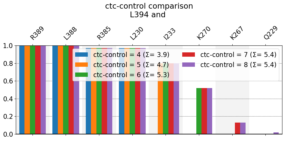
n is simply the number of reported bars: four blue ones, five orange ones, six green ones, seven red ones and eight purple ones. \(\Sigma\) is just the sum of the heights of all bars and is thus an estimate of the average number of neighbors that are being reported (at this cutoff). A couple of observations:
The relation of \(\Sigma\) with n is straightforward: as n grows, so does \(\Sigma\), although it grows slower with each n until it barely changes, given that the last bars it sums over are negligible. In other words, summing over the last purple bar (barely visible) for
Q229doesn’t really change \(\Sigma\) much.Hence, for a fixed cutoff, there’s an upper bond to \(\Sigma\) (\(\Sigma\leq\Sigma_t\)), because the total average number of neighbors, \(\Sigma_t\), of a given residue, over a given dataset, is determined by the used cutoff only. The
ctc_controlparameter simply determines how many neighbors get actually reported.Please note that for very small datasets, like one single pdb file, the word frequency doesn’t really have a defined meaning, so that, for this cases, it is better to use
ctc_control=1.0(more on this below).In cases where
mdciaois used to look for the neighborhood of just one residue, there’s a sensible number of residues to choose (somewhere between 5 and 10), because usually that’s how many interactions a residue will have (please note, this doesn’t necessary hold for elongated ligands, lipids, acid chains etc).
mdciao writes out the percentage of \(\Sigma_t\) captured by the reported contacts, so that the user can decide whether to increase n or not. For each of the iterations above, here are terminal-output reporting precisely that:
ctc_control = 4
The following 4 contacts capture 3.94 (~72%) of the total frequency 5.43 (over 9 contacts with nonzero frequency at 4.50 Angstrom).
As orientation value, the first 6 ctcs already capture 90.0% of 5.43.
The 6-th contact has a frequency of 0.52.
  freq    label      residues  fragments   sum
1  1.00  L394 - L388  353 - 347    0 - 0   1.00
2  1.00  L394 - R389  353 - 348    0 - 0   2.00
3  0.97  L394 - L230  353 - 957    0 - 3   2.97
4  0.97  L394 - R385  353 - 344    0 - 0   3.94
The intention is to report how much of \(\Sigma_t\) has been captured using 3 contacts (~72%), and how many would be needed to capture most (90%) of it (6 contacts). The actual value \(\Sigma_t\) is reported immediately after (total frequency 5.43). You will notice that the value 5.43 doesn’t change as we increase n in the reports below. The 9 contacts with nonzero frequency at 4.50 Angstrom is just telling that only 9 residue-pairs were closer than distance the distance cutoff in
at least %1 of the data (see the parameter min_freq=0.01).
So, as we increase n, the listed contacts grows and the reported percentage grows, but all the rest stays the same
ctc_control = 5
The following 5 contacts capture 4.74 (~87%) of the total frequency 5.43 (over 9 contacts with nonzero frequency at 4.50 Angstrom).
As orientation value, the first 6 ctcs already capture 90.0% of 5.43.
The 6-th contact has a frequency of 0.52.
  freq    label      residues  fragments   sum
1  1.00  L394 - L388  353 - 347    0 - 0   1.00
2  1.00  L394 - R389  353 - 348    0 - 0   2.00
3  0.97  L394 - L230  353 - 957    0 - 3   2.97
4  0.97  L394 - R385  353 - 344    0 - 0   3.94
5  0.80  L394 - I233  353 - 960    0 - 3   4.74
ctc_control = 6
The following 6 contacts capture 5.26 (~97%) of the total frequency 5.43 (over 9 contacts with nonzero frequency at 4.50 Angstrom).
As orientation value, the first 6 ctcs already capture 90.0% of 5.43.
The 6-th contact has a frequency of 0.52.
  freq    label      residues  fragments   sum
1  1.00  L394 - L388  353 - 347    0 - 0   1.00
2  1.00  L394 - R389  353 - 348    0 - 0   2.00
3  0.97  L394 - L230  353 - 957    0 - 3   2.97
4  0.97  L394 - R385  353 - 344    0 - 0   3.94
5  0.80  L394 - I233  353 - 960    0 - 3   4.74
6  0.52  L394 - K270  353 - 972    0 - 3   5.26
ctc_control = 7
The following 7 contacts capture 5.39 (~99%) of the total frequency 5.43 (over 9 contacts with nonzero frequency at 4.50 Angstrom).
As orientation value, the first 6 ctcs already capture 90.0% of 5.43.
The 6-th contact has a frequency of 0.52.
  freq    label      residues  fragments   sum
1  1.00  L394 - L388  353 - 347    0 - 0   1.00
2  1.00  L394 - R389  353 - 348    0 - 0   2.00
3  0.97  L394 - L230  353 - 957    0 - 3   2.97
4  0.97  L394 - R385  353 - 344    0 - 0   3.94
5  0.80  L394 - I233  353 - 960    0 - 3   4.74
6  0.52  L394 - K270  353 - 972    0 - 3   5.26
7  0.13  L394 - K267  353 - 969    0 - 3   5.39
ctc_control = 8
The following 8 contacts capture 5.41 (~100%) of the total frequency 5.43 (over 9 contacts with nonzero frequency at 4.50 Angstrom).
As orientation value, the first 6 ctcs already capture 90.0% of 5.43.
The 6-th contact has a frequency of 0.52.
  freq    label      residues  fragments   sum
1  1.00  L394 - L388  353 - 347    0 - 0   1.00
2  1.00  L394 - R389  353 - 348    0 - 0   2.00
3  0.97  L394 - L230  353 - 957    0 - 3   2.97
4  0.97  L394 - R385  353 - 344    0 - 0   3.94
5  0.80  L394 - I233  353 - 960    0 - 3   4.74
6  0.52  L394 - K270  353 - 972    0 - 3   5.26
7  0.13  L394 - K267  353 - 969    0 - 3   5.39
8  0.02  L394 - Q229  353 - 956    0 - 3   5.41
Controlling with fractions
Additionally, the upper bond itself, \(\Sigma_t\), can be used as a reference for controlling how many contacts get reported. So, instead of specifying an absolute number (n = 4,5,6…), one can specify a relative number, i.e. a fraction of \(\Sigma_t\) to be reported.
This way, regardless of the actual number of involved contacts, one can choose to report most of them. In the example below, we choose to report 90% of the total number of average neighbors, which, as we know from above, is achieved with 6 contacts. To avoid introducing a new parameter, mdciao knows that if ctc_control is an integer (1, 2, 3…), the user means these many contacts, whereas if ctc_control is between 0 and 1 (.50 for 50%, .9 for 90% etc) the user wants that
fraction of \(\Sigma_t\):
[6]:
mdciao.cli.residue_neighborhoods("L394",traj,
                                 short_AA_names=True,
                                 ctc_cutoff_Ang=ctc_cutoff_Ang,
                                 ctc_control=1.0,
                                 figures=False,
                                 fragment_names=None,
                                 no_disk=False,
                                 );
Will compute contact frequencies for (1 items):
<mdtraj.Trajectory with 280 frames, 8384 atoms, 1044 residues, and unitcells>
 with a stride of 1 frames
Using method 'lig_resSeq+' these fragments were found
fragment 0 with    354 AAs     LEU4 (   0) -   LEU394 (353 ) (0) resSeq jumps
fragment 1 with    340 AAs     GLN1 ( 354) -   ASN340 (693 ) (1)
fragment 2 with     66 AAs     ALA2 ( 694) -    PHE67 (759 ) (2)
fragment 3 with    283 AAs    GLU30 ( 760) -   LEU340 (1042) (3) resSeq jumps
fragment 4 with      1 AAs   P0G395 (1043) -   P0G395 (1043) (4)

Will compute neighborhoods for the residues
L394
excluding 4 nearest neighbors

   residue      residx    fragment      resSeq
    LEU394         353           0         394

Performing a first pass on 1039 residue pairs to compute lower bounds on residue-residue distances via residue-COM distances:
Reduced to only 45 residue pairs for the computation of actual residue-residue distances:
L394:
The following 9 contacts capture 6.09 (~100%) of the total frequency 6.09 (over 11 contacts with nonzero frequency at 5.00 Angstrom).
As orientation value, the first 6 ctcs already capture 90.0% of 6.09.
The 6-th contact has a frequency of 0.64.
   freq    label      residues  fragments   sum
1  1.00  L394 - R389  353 - 348    0 - 0   1.00
2  1.00  L394 - L388  353 - 347    0 - 0   2.00
3  1.00  L394 - L230  353 - 957    0 - 3   3.00
4  1.00  L394 - R385  353 - 344    0 - 0   3.99
5  0.98  L394 - I233  353 - 960    0 - 3   4.97
6  0.64  L394 - K270  353 - 972    0 - 3   5.60
7  0.36  L394 - K267  353 - 969    0 - 3   5.97
8  0.09  L394 - Q229  353 - 956    0 - 3   6.05
9  0.03  L394 - A226  353 - 953    0 - 3   6.09
The following files have been created:
./neighborhood.LEU394@5.0_Ang.dat
Which control-mode to choose (fraction or integers) is up to the user:
For compactness, limiting the output with integers can avoid huge outputs, but might leave out some interesting stuff.
For completeness, choosing
ctc_control = 1.0will ensure that any-residue under the cutoff (regardless of its frequency) will be reported, but might fill the reports with “long tails” of many residues with very low frequencies (see below).
n_nearest
Another way in which mdciao is choosing which contacts to show is through excluding nearest neighbors, i.e. residues that are predictably going to be under the cutoff simply because they are bonded neighbors of the residue in question.
In our example, for L394 these would be residues 395 and 393 (first bonded) 396 and 392 (second bonded) and so on (except, in this particular L394 case, since it’s a terminal residue, we only get 393, 392 etc).
The default value that mdciao has for this parameter is n_nearest=4, which is approximately one \(\alpha\)-helix turn away. The intention is to avoid reporting residues in the helix-turns immediately before and immediately after the residue.
Let’s see the effect of varying this parameter:
[7]:
%%capture
n_nearests = [0, 1, 2, 3, 4]
for n_nearest in n_nearests:
    n = mdciao.cli.residue_neighborhoods("L394",traj,
                                     short_AA_names=True,
                                     ctc_control=20,
                                     n_nearest=n_nearest,
                                     figures=False,
                                     no_disk=False,
                                     output_desc='neighborhood.n_nearest_%u'%n_nearest)
[8]:
mdciao.cli.compare({"n_n = %u"%key : "neighborhood.n_nearest_%u.LEU394@frag0@%2.1f_Ang.dat"%(key,4.5)
                    for key in n_nearests},
                   anchor="L394",
                   sort_by="residue",
                   title="n_neighbors comparison");
These interactions are not shared:
E392, L393
Their cumulative ctc freq is 3.00.
Created files
freq_comparison.pdf
freq_comparison.xlsx
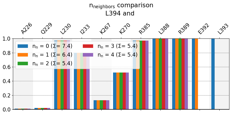
- The bars:Since we’ve sorted the frequency bars by increasing residue number, the closer to the right the bar is, the closer (in space) to
L394we are. Hence,L394’s immediate bonded neighbor,L393, only gets a bar whenn=0(no excuded neighbors, blue bar). Accordingly, next the residue after that,E392, only gets a bar withn=0orn=1, else it’s excluded. SinceL393is covalently bonded toL394, andL392is covalently bonded toL392, there’s a strong expectation for these residue to be near each other, so these frequencies are not very informative. If you’re wondering what’s with positions 390 and 391, there’s a bend in the C-terminus of the alpha helix 5 (TYR391points away fromL394throughout the simulation) so they do not appear on the report regardless. - The legend:We can see also here that, the lower
n_neighbors, i.e. the less neighbors we exclude, the higher the \(\Sigma\) value. So, asn_neighborsgoes up, these two bars get hidden, and the graph doesn’t change anymore.
Interfaces: ctc_control and min_freq
When computing interfaces between two different groups of residues using mdciao.cli.interface, one can set ctc_control=1.0 and min_freq=O to force mdciao to report all nonzero frequencies. This means any and all residue pairs that, at any given point in time, might have been at a distance >= ctc_cutoff_Ang (even if was just for one frame) will be
reported.
After reporting the most relevant contacts, this approach typically reports also a high number of very low frequency contacts, i.e. a long tail of very low frequency contacts, in particular for large interfaces (more on this tail below).
First, we take a look at the full list of contacts by using: * ctc_control=1.0 * min_freq=0
[9]:
intf = mdciao.cli.interface("mdciao_example/traj.xtc", topology="mdciao_example/top.pdb",
                            no_disk=True, interface_selection_1=[0], interface_selection_2=[1],
                            ctc_control=1.0,
                            min_freq=0,
                            figures=False);
intf.plot_freqs_as_bars(4.5, shorten_AAs=True, defrag="@", cumsum=True);
Will compute contact frequencies for trajectories:
mdciao_example/traj.xtc
 with a stride of 1 frames
Using method 'lig_resSeq+' these fragments were found
fragment 0 with    354 AAs     LEU4 (   0) -   LEU394 (353 ) (0) resSeq jumps
fragment 1 with    340 AAs     GLN1 ( 354) -   ASN340 (693 ) (1)
fragment 2 with     66 AAs     ALA2 ( 694) -    PHE67 (759 ) (2)
fragment 3 with    283 AAs    GLU30 ( 760) -   LEU340 (1042) (3) resSeq jumps
fragment 4 with      1 AAs   P0G395 (1043) -   P0G395 (1043) (4)
Select group 1: 0
Select group 2: 1

Will look for contacts in the interface between fragments
0
and
1.

Performing a first pass on the 120360 group_1-group_2 residue pairs to compute lower bounds on residue-residue distances via residue-COM distances.
Reduced to only 1153 (from 120360) residue pairs for the computation of actual residue-residue distances:
The following 138 contacts capture 74.50 (~100%) of the total frequency 74.50 (over 138 contacts with nonzero frequency at 4.50 Angstrom).
As orientation value, the first 73 ctcs already capture 90.0% of 74.50.
The 73-th contact has a frequency of 0.57.

     freq    label      residues  fragments   sum
1    1.00  I26  - K89    22 - 442    0 - 1    1.00
2    1.00  R228 - G162  194 - 515    0 - 1    2.00
3    1.00  R228 - D186  194 - 539    0 - 1    3.00
4    1.00  Q227 - Y145  193 - 498    0 - 1    4.00
5    1.00  Y37  - L55    33 - 408    0 - 1    5.00
6    1.00  K233 - N230  199 - 583    0 - 1    6.00
7    1.00  K233 - D246  199 - 599    0 - 1    7.00
8    1.00  D33  - K78    29 - 431    0 - 1    8.00
9    1.00  F238 - L117  204 - 470    0 - 1    9.00
10   1.00  F238 - W99   204 - 452    0 - 1   10.00
11   1.00  Q227 - N119  193 - 472    0 - 1   11.00
12   1.00  L30  - G53    26 - 406    0 - 1   12.00
13   1.00  R201 - R96   169 - 449    0 - 1   13.00
14   1.00  N23  - N88    19 - 441    0 - 1   14.00
15   1.00  N23  - K89    19 - 442    0 - 1   15.00
16   1.00  F222 - L117  188 - 470    0 - 1   16.00
17   1.00  F222 - W99   188 - 452    0 - 1   17.00
18   1.00  C237 - W99   203 - 452    0 - 1   18.00
19   1.00  E27  - K89    23 - 442    0 - 1   19.00
20   1.00  C237 - Q75   203 - 428    0 - 1   20.00
21   1.00  C237 - K57   203 - 410    0 - 1   21.00
22   1.00  I26  - A92    22 - 445    0 - 1   22.00
23   1.00  D240 - K57   206 - 410    0 - 1   23.00
24   1.00  Q236 - Y59   202 - 412    0 - 1   24.00
25   1.00  K233 - D290  199 - 643    0 - 1   24.99
26   1.00  C237 - Y59   203 - 412    0 - 1   25.99
27   1.00  Q236 - W332  202 - 685    0 - 1   26.99
28   1.00  Q19  - N88    15 - 441    0 - 1   27.98
29   0.99  I172 - E130  140 - 483    0 - 1   28.97
30   0.99  Q227 - L117  193 - 470    0 - 1   29.97
31   0.99  R20  - N88    16 - 441    0 - 1   30.96
32   0.99  K34  - L55    30 - 408    0 - 1   31.95
33   0.99  Q236 - K57   202 - 410    0 - 1   32.94
34   0.99  Q19  - T86    15 - 439    0 - 1   33.92
35   0.98  A22  - K89    18 - 442    0 - 1   34.90
36   0.98  R228 - Y145  194 - 498    0 - 1   35.89
37   0.98  F208 - D118  174 - 471    0 - 1   36.87
38   0.98  C237 - L117  203 - 470    0 - 1   37.85
39   0.98  W281 - R314  240 - 667    0 - 1   38.82
40   0.98  I172 - N132  140 - 485    0 - 1   39.80
41   0.98  W234 - Y145  200 - 498    0 - 1   40.77
42   0.97  Q19  - D83    15 - 436    0 - 1   41.74
43   0.97  R42  - W99    38 - 452    0 - 1   42.71
44   0.97  R42  - D76    38 - 429    0 - 1   43.69
45   0.96  D33  - L55    29 - 408    0 - 1   44.65
46   0.96  W234 - L117  200 - 470    0 - 1   45.61
47   0.96  I26  - H91    22 - 444    0 - 1   46.58
48   0.96  E209 - S98   175 - 451    0 - 1   47.54
49   0.94  I172 - R134  140 - 487    0 - 1   48.47
50   0.93  F208 - L117  174 - 470    0 - 1   49.41
51   0.93  Q227 - G144  193 - 497    0 - 1   50.34
52   0.93  N239 - W332  205 - 685    0 - 1   51.27
53   0.92  C237 - M101  203 - 454    0 - 1   52.19
54   0.91  Q19  - R68    15 - 421    0 - 1   53.10
55   0.90  Q19  - V90    15 - 443    0 - 1   54.01
56   0.90  Q170 - R129  138 - 482    0 - 1   54.91
57   0.89  G226 - T143  192 - 496    0 - 1   55.80
58   0.89  W281 - W332  240 - 685    0 - 1   56.69
59   0.87  F208 - N119  174 - 472    0 - 1   57.56
60   0.86  L30  - K89    26 - 442    0 - 1   58.42
61   0.83  Q170 - G131  138 - 484    0 - 1   59.25
62   0.81  A22  - V90    18 - 443    0 - 1   60.06
63   0.80  I26  - V90    22 - 443    0 - 1   60.86
64   0.77  I172 - G131  140 - 484    0 - 1   61.63
65   0.75  E16  - T86    12 - 439    0 - 1   62.39
66   0.70  K233 - Y59   199 - 412    0 - 1   63.09
67   0.66  Q170 - E130  138 - 483    0 - 1   63.75
68   0.63  F222 - D118  188 - 471    0 - 1   64.38
69   0.63  I207 - D118  173 - 471    0 - 1   65.01
70   0.62  L30  - L55    26 - 408    0 - 1   65.63
71   0.61  E15  - R68    11 - 421    0 - 1   66.24
72   0.59  E16  - N88    12 - 441    0 - 1   66.83
73   0.57  W234 - M101  200 - 454    0 - 1   67.40
74   0.54  R232 - D228  198 - 581    0 - 1   67.94
75   0.52  E209 - W99   175 - 452    0 - 1   68.46
76   0.50  Q236 - D290  202 - 643    0 - 1   68.96
77   0.41  E209 - R96   175 - 449    0 - 1   69.38
78   0.39  Q19  - K89    15 - 442    0 - 1   69.76
79   0.37  V241 - W99   207 - 452    0 - 1   70.13
80   0.30  H220 - W99   186 - 452    0 - 1   70.44
81   0.29  L171 - E130  139 - 483    0 - 1   70.72
82   0.26  I207 - I120  173 - 473    0 - 1   70.99
83   0.23  R20  - T86    16 - 439    0 - 1   71.22
84   0.22  K233 - G272  199 - 625    0 - 1   71.44
85   0.22  R201 - E138  169 - 491    0 - 1   71.65
86   0.21  Q227 - T143  193 - 496    0 - 1   71.86
87   0.19  G226 - N119  192 - 472    0 - 1   72.05
88   0.17  R42  - A56    38 - 409    0 - 1   72.22
89   0.16  Q12  - T86     8 - 439    0 - 1   72.37
90   0.14  R42  - L55    38 - 408    0 - 1   72.51
91   0.14  L43  - W99    39 - 452    0 - 1   72.65
92   0.13  R232 - D246  198 - 599    0 - 1   72.78
93   0.12  R232 - C204  198 - 557    0 - 1   72.90
94   0.10  E101 - N132   69 - 485    0 - 1   73.00
95   0.10  E15  - T86    11 - 439    0 - 1   73.10
96   0.09  R42  - S98    38 - 451    0 - 1   73.19
97   0.09  Q12  - Y85     8 - 438    0 - 1   73.28
98   0.09  D173 - R134  141 - 487    0 - 1   73.36
99   0.08  R42  - Q75    38 - 428    0 - 1   73.44
100  0.06  Q170 - T128  138 - 481    0 - 1   73.51
101  0.06  Q12  - R68     8 - 421    0 - 1   73.57
102  0.06  N239 - K57   205 - 410    0 - 1   73.63
103  0.06  N239 - N313  205 - 666    0 - 1   73.69
104  0.05  R228 - D163  194 - 516    0 - 1   73.74
105  0.05  L30  - R52    26 - 405    0 - 1   73.79
106  0.05  V224 - L117  190 - 470    0 - 1   73.84
107  0.05  Q19  - L69    15 - 422    0 - 1   73.88
108  0.04  R20  - T87    16 - 440    0 - 1   73.92
109  0.04  W234 - Y59   200 - 412    0 - 1   73.97
110  0.04  K233 - I273  199 - 626    0 - 1   74.01
111  0.04  G226 - G144  192 - 497    0 - 1   74.05
112  0.04  R232 - D186  198 - 539    0 - 1   74.10
113  0.04  C174 - R134  142 - 487    0 - 1   74.14
114  0.04  C174 - N132  142 - 485    0 - 1   74.18
115  0.04  F238 - K57   204 - 410    0 - 1   74.21
116  0.04  I26  - I80    22 - 433    0 - 1   74.25
117  0.03  K233 - M188  199 - 541    0 - 1   74.28
118  0.03  D173 - E130  141 - 483    0 - 1   74.31
119  0.03  F222 - S98   188 - 451    0 - 1   74.34
120  0.01  R201 - L95   169 - 448    0 - 1   74.35
121  0.01  K233 - M101  199 - 454    0 - 1   74.37
122  0.01  Q236 - R314  202 - 667    0 - 1   74.38
123  0.01  N23  - T87    19 - 440    0 - 1   74.40
124  0.01  Q170 - N132  138 - 485    0 - 1   74.41
125  0.01  N167 - R129  135 - 482    0 - 1   74.43
126  0.01  L171 - R129  139 - 482    0 - 1   74.44
127  0.01  R232 - Y145  198 - 498    0 - 1   74.45
128  0.01  M221 - W99   187 - 452    0 - 1   74.45
129  0.01  K34  - G53    30 - 406    0 - 1   74.46
130  0.01  E209 - S97   175 - 450    0 - 1   74.47
131  0.01  R280 - R314  239 - 667    0 - 1   74.48
132  0.01  D240 - A56   206 - 409    0 - 1   74.48
133  0.00  R228 - G144  194 - 497    0 - 1   74.49
134  0.00  Q29  - A92    25 - 445    0 - 1   74.49
135  0.00  L30  - I80    26 - 433    0 - 1   74.49
136  0.00  D240 - W99   206 - 452    0 - 1   74.50
137  0.00  Q236 - Q75   202 - 428    0 - 1   74.50
138  0.00  L171 - R134  139 - 487    0 - 1   74.50

   label  freq
1   C237  5.90
2    Q19  5.20
3   Q227  4.13
4   K233  4.01
5    I26  3.80
6   I172  3.68
7   Q236  3.50
8   R228  3.04
9   F208  2.79
10  F222  2.66
11  W234  2.55
12   L30  2.54
13  Q170  2.46
14   R42  2.42
15  F238  2.04
16   N23  2.01
17   D33  1.96
18  E209  1.90
19  W281  1.86
20   A22  1.79
21   E16  1.34
22   R20  1.26
23  R201  1.23
24  G226  1.12
25  N239  1.04
26  D240  1.01
27   Y37  1.00
28   E27  1.00
29   K34  1.00
30  I207  0.90
31  R232  0.84
32   E15  0.71
33  V241  0.37
34   Q12  0.31
35  L171  0.30
36  H220  0.30
37   L43  0.14
38  D173  0.11
39  E101  0.10
40  C174  0.08
41  V224  0.05
42  N167  0.01
43  M221  0.01
44  R280  0.01
45   Q29  0.00

   label  freq
1   L117  5.91
2    W99  5.31
3    K89  5.23
4    L55  3.71
5    N88  3.58
6    K57  3.08
7   Y145  2.97
8   W332  2.81
9    Y59  2.74
10   V90  2.51
11  D118  2.25
12   T86  2.22
13  N119  2.06
14  E130  1.97
15  G131  1.60
16   R68  1.59
17  M101  1.51
18  D290  1.50
19   R96  1.41
20  D246  1.13
21  N132  1.13
22  T143  1.10
23   Q75  1.08
24   S98  1.08
25  R134  1.07
26  D186  1.04
27   G53  1.01
28   A92  1.00
29  G162  1.00
30  N230  1.00
31   K78  1.00
32  R314  1.00
33  G144  0.98
34   D83  0.97
35   D76  0.97
36   H91  0.96
37  R129  0.92
38  D228  0.54
39  I120  0.26
40  G272  0.22
41  E138  0.22
42   A56  0.18
43  C204  0.12
44   Y85  0.09
45  T128  0.06
46  N313  0.06
47   T87  0.06
48  D163  0.05
49   R52  0.05
50   L69  0.05
51  I273  0.04
52   I80  0.04
53  M188  0.03
54   L95  0.01
55   S97  0.01

In the graph (double click to enlarge), we note the long tail of the bar-plot as we move to the right. Where exactly should one stop to pay attention can’t be really answered numercally alone. mdciao tries to provide hints as to what might be sane values, e.g, the log reports:
The following 138 contacts capture 74.50 (~100%) of the total frequency 74.50 (over 138 contacts with nonzero frequency at 4.50 Angstrom).
As orientation value, the first 73 ctcs already capture 90.0% of 74.50.
The 73-th contact has a frequency of 0.57
ctc_control=1.0, min_freq=0.0, are capturing 100% of anything there is to report.mdciao looks for how many contacts one would need to capture 90% of that 100%, and the in this case the number is 73.mdciao informs the user of the frequency value of that last contact at 90%. In this case, that value (0.57 i.e. 57%) is, in this case, too high to be discarded.Hence, as a compromise between reporting everything or risking truncating too early, mdciao sets by default min_freq=0.10, i.e. contacts formed less than 10% of the time are simply not included in the returned ContactGroup. The long tail is contained in the above report, nevertheless:
[10]:
intf = mdciao.cli.interface("mdciao_example/traj.xtc", topology="mdciao_example/top.pdb",
                            no_disk=True, interface_selection_1=[0], interface_selection_2=[1],
                            ctc_control=1.0,
                            figures=False);
intf.plot_freqs_as_bars(4.5, shorten_AAs=True, defrag="@", cumsum=True);
Will compute contact frequencies for trajectories:
mdciao_example/traj.xtc
 with a stride of 1 frames
Using method 'lig_resSeq+' these fragments were found
fragment 0 with    354 AAs     LEU4 (   0) -   LEU394 (353 ) (0) resSeq jumps
fragment 1 with    340 AAs     GLN1 ( 354) -   ASN340 (693 ) (1)
fragment 2 with     66 AAs     ALA2 ( 694) -    PHE67 (759 ) (2)
fragment 3 with    283 AAs    GLU30 ( 760) -   LEU340 (1042) (3) resSeq jumps
fragment 4 with      1 AAs   P0G395 (1043) -   P0G395 (1043) (4)
Select group 1: 0
Select group 2: 1

Will look for contacts in the interface between fragments
0
and
1.

Performing a first pass on the 120360 group_1-group_2 residue pairs to compute lower bounds on residue-residue distances via residue-COM distances.
Reduced to only 1153 (from 120360) residue pairs for the computation of actual residue-residue distances:
The following 93 contacts capture 72.90 (~98%) of the total frequency 74.50 (over 138 contacts with nonzero frequency at 4.50 Angstrom).
As orientation value, the first 73 ctcs already capture 90.0% of 74.50.
The 73-th contact has a frequency of 0.57.

    freq    label      residues  fragments   sum
1   1.00  I26  - K89    22 - 442    0 - 1    1.00
2   1.00  R228 - G162  194 - 515    0 - 1    2.00
3   1.00  R228 - D186  194 - 539    0 - 1    3.00
4   1.00  Q227 - Y145  193 - 498    0 - 1    4.00
5   1.00  Y37  - L55    33 - 408    0 - 1    5.00
6   1.00  K233 - N230  199 - 583    0 - 1    6.00
7   1.00  K233 - D246  199 - 599    0 - 1    7.00
8   1.00  D33  - K78    29 - 431    0 - 1    8.00
9   1.00  F238 - L117  204 - 470    0 - 1    9.00
10  1.00  F238 - W99   204 - 452    0 - 1   10.00
11  1.00  Q227 - N119  193 - 472    0 - 1   11.00
12  1.00  L30  - G53    26 - 406    0 - 1   12.00
13  1.00  R201 - R96   169 - 449    0 - 1   13.00
14  1.00  N23  - N88    19 - 441    0 - 1   14.00
15  1.00  N23  - K89    19 - 442    0 - 1   15.00
16  1.00  F222 - L117  188 - 470    0 - 1   16.00
17  1.00  F222 - W99   188 - 452    0 - 1   17.00
18  1.00  C237 - W99   203 - 452    0 - 1   18.00
19  1.00  E27  - K89    23 - 442    0 - 1   19.00
20  1.00  C237 - Q75   203 - 428    0 - 1   20.00
21  1.00  C237 - K57   203 - 410    0 - 1   21.00
22  1.00  I26  - A92    22 - 445    0 - 1   22.00
23  1.00  D240 - K57   206 - 410    0 - 1   23.00
24  1.00  Q236 - Y59   202 - 412    0 - 1   24.00
25  1.00  K233 - D290  199 - 643    0 - 1   24.99
26  1.00  C237 - Y59   203 - 412    0 - 1   25.99
27  1.00  Q236 - W332  202 - 685    0 - 1   26.99
28  1.00  Q19  - N88    15 - 441    0 - 1   27.98
29  0.99  I172 - E130  140 - 483    0 - 1   28.97
30  0.99  Q227 - L117  193 - 470    0 - 1   29.97
31  0.99  R20  - N88    16 - 441    0 - 1   30.96
32  0.99  K34  - L55    30 - 408    0 - 1   31.95
33  0.99  Q236 - K57   202 - 410    0 - 1   32.94
34  0.99  Q19  - T86    15 - 439    0 - 1   33.92
35  0.98  A22  - K89    18 - 442    0 - 1   34.90
36  0.98  R228 - Y145  194 - 498    0 - 1   35.89
37  0.98  F208 - D118  174 - 471    0 - 1   36.87
38  0.98  C237 - L117  203 - 470    0 - 1   37.85
39  0.98  W281 - R314  240 - 667    0 - 1   38.82
40  0.98  I172 - N132  140 - 485    0 - 1   39.80
41  0.98  W234 - Y145  200 - 498    0 - 1   40.77
42  0.97  Q19  - D83    15 - 436    0 - 1   41.74
43  0.97  R42  - W99    38 - 452    0 - 1   42.71
44  0.97  R42  - D76    38 - 429    0 - 1   43.69
45  0.96  D33  - L55    29 - 408    0 - 1   44.65
46  0.96  W234 - L117  200 - 470    0 - 1   45.61
47  0.96  I26  - H91    22 - 444    0 - 1   46.58
48  0.96  E209 - S98   175 - 451    0 - 1   47.54
49  0.94  I172 - R134  140 - 487    0 - 1   48.47
50  0.93  F208 - L117  174 - 470    0 - 1   49.41
51  0.93  Q227 - G144  193 - 497    0 - 1   50.34
52  0.93  N239 - W332  205 - 685    0 - 1   51.27
53  0.92  C237 - M101  203 - 454    0 - 1   52.19
54  0.91  Q19  - R68    15 - 421    0 - 1   53.10
55  0.90  Q19  - V90    15 - 443    0 - 1   54.01
56  0.90  Q170 - R129  138 - 482    0 - 1   54.91
57  0.89  G226 - T143  192 - 496    0 - 1   55.80
58  0.89  W281 - W332  240 - 685    0 - 1   56.69
59  0.87  F208 - N119  174 - 472    0 - 1   57.56
60  0.86  L30  - K89    26 - 442    0 - 1   58.42
61  0.83  Q170 - G131  138 - 484    0 - 1   59.25
62  0.81  A22  - V90    18 - 443    0 - 1   60.06
63  0.80  I26  - V90    22 - 443    0 - 1   60.86
64  0.77  I172 - G131  140 - 484    0 - 1   61.63
65  0.75  E16  - T86    12 - 439    0 - 1   62.39
66  0.70  K233 - Y59   199 - 412    0 - 1   63.09
67  0.66  Q170 - E130  138 - 483    0 - 1   63.75
68  0.63  F222 - D118  188 - 471    0 - 1   64.38
69  0.63  I207 - D118  173 - 471    0 - 1   65.01
70  0.62  L30  - L55    26 - 408    0 - 1   65.63
71  0.61  E15  - R68    11 - 421    0 - 1   66.24
72  0.59  E16  - N88    12 - 441    0 - 1   66.83
73  0.57  W234 - M101  200 - 454    0 - 1   67.40
74  0.54  R232 - D228  198 - 581    0 - 1   67.94
75  0.52  E209 - W99   175 - 452    0 - 1   68.46
76  0.50  Q236 - D290  202 - 643    0 - 1   68.96
77  0.41  E209 - R96   175 - 449    0 - 1   69.38
78  0.39  Q19  - K89    15 - 442    0 - 1   69.76
79  0.37  V241 - W99   207 - 452    0 - 1   70.13
80  0.30  H220 - W99   186 - 452    0 - 1   70.44
81  0.29  L171 - E130  139 - 483    0 - 1   70.72
82  0.26  I207 - I120  173 - 473    0 - 1   70.99
83  0.23  R20  - T86    16 - 439    0 - 1   71.22
84  0.22  K233 - G272  199 - 625    0 - 1   71.44
85  0.22  R201 - E138  169 - 491    0 - 1   71.65
86  0.21  Q227 - T143  193 - 496    0 - 1   71.86
87  0.19  G226 - N119  192 - 472    0 - 1   72.05
88  0.17  R42  - A56    38 - 409    0 - 1   72.22
89  0.16  Q12  - T86     8 - 439    0 - 1   72.37
90  0.14  R42  - L55    38 - 408    0 - 1   72.51
91  0.14  L43  - W99    39 - 452    0 - 1   72.65
92  0.13  R232 - D246  198 - 599    0 - 1   72.78
93  0.12  R232 - C204  198 - 557    0 - 1   72.90

   label  freq
1   C237  5.90
2    Q19  5.15
3   Q227  4.13
4   K233  3.92
5    I26  3.76
6   I172  3.68
7   Q236  3.48
8   R228  2.98
9   F208  2.79
10  F222  2.63
11  W234  2.51
12   L30  2.49
13  Q170  2.39
14   R42  2.25
15  F238  2.00
16   N23  2.00
17   D33  1.96
18  E209  1.89
19  W281  1.86
20   A22  1.79
21   E16  1.34
22   R20  1.22
23  R201  1.22
24  G226  1.08
25   Y37  1.00
26   E27  1.00
27  D240  1.00
28   K34  0.99
29  N239  0.93
30  I207  0.90
31  R232  0.79
32   E15  0.61
33  V241  0.37
34  H220  0.30
35  L171  0.29
36   Q12  0.16
37   L43  0.14

   label  freq
1   L117  5.87
2    W99  5.30
3    K89  5.23
4    L55  3.71
5    N88  3.58
6    K57  2.99
7   Y145  2.96
8   W332  2.81
9    Y59  2.70
10   V90  2.51
11  D118  2.25
12   T86  2.12
13  N119  2.06
14  E130  1.94
15  G131  1.60
16   R68  1.52
17  D290  1.50
18  M101  1.49
19   R96  1.41
20  D246  1.13
21  T143  1.10
22  G162  1.00
23  D186  1.00
24  N230  1.00
25   K78  1.00
26   G53  1.00
27   Q75  1.00
28   A92  1.00
29  R314  0.98
30  N132  0.98
31   D83  0.97
32   D76  0.97
33   H91  0.96
34   S98  0.96
35  R134  0.94
36  G144  0.93
37  R129  0.90
38  D228  0.54
39  I120  0.26
40  G272  0.22
41  E138  0.22
42   A56  0.17
43  C204  0.12

The output
The following 93 contacts capture 72.90 (~98%) of the total frequency 74.50 (over 138 contacts with nonzero frequency at 4.50 Angstrom).
As orientation value, the first 73 ctcs already capture 90.0% of 74.50.
The 73-th contact has a frequency of 0.57
let’s us know that ignoring frequencies < .1 reduces the full list from 138 to 93 entries while keeping ca 98% of \(\Sigma_t\). In this case, even if we have ctc_control=1.0 we don’t get 100% of the freqs reported (only 98%) because the min_freq=0.1 (default value) is causing the loss of %2 of contacts all of which have frequencies below 10%.
Interfaces: self_interface
From the docs of mdciao.cli.interface:
Note
----
If your definitions of `interface_selection_1` and
`interface_selection_2` lead to some overlap between
the interface members (see below), mdciao's default
is to ignore contact pairs within the same fragment.
E.g., in the context of a GPCR, computing
"TM3" vs "TM*" ("TM3" vs "all TMs") won't include
TM3-TM3 contacts by default. To include these
(or equivalent) contacts set `self_interface` = True.

Another example could be computing the interface of
C-terminus of a receptor with the entire receptor,
where it might be useful to include the contacts of
the C-terminus with itself.

When using `self_interface` = True, it's advisable to
increase `n_nearest`, since otherwise neighboring
residues of the shared set (the TM3-TM3 or the Cterm-Cterm)
will always appear as formed.
We can compute the self contacts of the $:nbsphinx-math:`alpha`$5-helix of the G-protein. Whereas most of the helix is straight, the C-terminal bends a bit backwards and interacts with itself:
[11]:
intf = mdciao.cli.interface("mdciao_example/traj.xtc", topology="mdciao_example/top.pdb",
                            fragments="consensus",accept_guess=True,
                            no_disk=True, interface_selection_1="G.H5", interface_selection_2="G.H5",
                            ctc_control=1.0,
                            GPCR_UniProt="adrb2_human",CGN_UniProt="gnas2_human",
                            self_interface=True,
                            #min_freq=0,
                            n_nearest=4,
                            figures=False)
intf.plot_freqs_as_bars(4.5, shorten_AAs=True, plot_atomtypes=True);
Will compute contact frequencies for trajectories:
mdciao_example/traj.xtc
 with a stride of 1 frames
Using method 'resSeq+' these fragments were found
fragment 0 with    354 AAs     LEU4 (   0) -   LEU394 (353 ) (0) resSeq jumps
fragment 1 with    340 AAs     GLN1 ( 354) -   ASN340 (693 ) (1)
fragment 2 with     66 AAs     ALA2 ( 694) -    PHE67 (759 ) (2)
fragment 3 with    284 AAs    GLU30 ( 760) -   P0G395 (1043) (3) resSeq jumps
No local file ./adrb2_human.xlsx found, checking online in
https://gpcrdb.org/services/residues/extended/adrb2_human ...done!
Please cite the following reference to the GPCRdb:
 * Kooistra et al, (2021) GPCRdb in 2021: Integrating GPCR sequence, structure and function
   Nucleic Acids Research 49, D335--D343
   https://doi.org/10.1093/nar/gkaa1080
For more information, call mdciao.nomenclature.references()
The GPCR-labels align best with fragments: [3] (first-last: GLU30-P0G395).

Mapping the GPCR fragments onto your topology:
 TM1  with     32 AAs    GLU30@1.29x29   ( 760) -    PHE61@1.60x60   (791 ) (TM1)
 ICL1 with      4 AAs    GLU62@12.48x48  ( 792) -    GLN65@12.51x51  (795 ) (ICL1)
 TM2  with     32 AAs    THR66@2.37x37   ( 796) -    LYS97@2.68x67   (827 ) (TM2)
 ECL1 with      4 AAs    MET98@23.49x49  ( 828) -   PHE101@23.52x52  (831 ) (ECL1)
 TM3  with     36 AAs   GLY102@3.21x21   ( 832) -   SER137@3.56x56   (867 ) (TM3)
 ICL2 with      8 AAs   PRO138@34.50x50  ( 868) -   LEU145@34.57x57  (875 ) (ICL2)
 TM4  with     27 AAs   THR146@4.38x38   ( 876) -   HIS172@4.64x64   (902 ) (TM4)
 ECL2 with     20 AAs   TRP173           ( 903) -   THR195           (922 ) (ECL2) resSeq jumps
 TM5  with     42 AAs   ASN196@5.35x36   ( 923) -   GLU237@5.76x76   (964 ) (TM5)
 ICL3 with      2 AAs   GLY238           ( 965) -   ARG239           (966 ) (ICL3)
 TM6  with     35 AAs   CYS265@6.27x27   ( 967) -   GLN299@6.61x61   (1001) (TM6)
 ECL3 with      4 AAs   ASP300           (1002) -   ILE303           (1005) (ECL3)
 TM7  with     25 AAs   ARG304@7.31x30   (1006) -   ARG328@7.55x55   (1030) (TM7)
 H8   with     12 AAs   SER329@8.47x47   (1031) -   LEU340@8.58x58   (1042) (H8)
No local file ./gnas2_human.xlsx found, checking online in
https://gpcrdb.org/services/residues/extended/gnas2_human ...done!
Please cite the following reference to the GPCRdb:
 * Kooistra et al, (2021) GPCRdb in 2021: Integrating GPCR sequence, structure and function
   Nucleic Acids Research 49, D335--D343
   https://doi.org/10.1093/nar/gkaa1080
Please cite the following reference to the CGN nomenclature:
 * Flock et al, (2015) Universal allosteric mechanism for G$\alpha$ activation by GPCRs
   Nature 2015 524:7564 524, 173--179
   https://doi.org/10.1038/nature14663
For more information, call mdciao.nomenclature.references()
The CGN-labels align best with fragments: [0] (first-last: LEU4-LEU394).

Mapping the CGN fragments onto your topology:
 G.HN   with     33 AAs     LEU4@G.HN.10   (   0) -    VAL36@G.HN.53   (32  ) (G.HN)
 G.hns1 with      3 AAs    TYR37@G.hns1.01 (  33) -    ALA39@G.hns1.03 (35  ) (G.hns1)
 G.S1   with      7 AAs    THR40@G.S1.01   (  36) -    LEU46@G.S1.07   (42  ) (G.S1)
 G.s1h1 with      6 AAs    GLY47@G.s1h1.01 (  43) -    GLY52@G.s1h1.06 (48  ) (G.s1h1)
 G.H1   with      7 AAs    LYS53@G.H1.01   (  49) -    GLN59@G.H1.07   (55  ) (G.H1)
 H.HA   with     26 AAs    LYS88@H.HA.04   (  56) -   LEU113@H.HA.29   (81  ) (H.HA)
 H.hahb with      9 AAs   VAL114@H.hahb.01 (  82) -   PRO122@H.hahb.09 (90  ) (H.hahb)
 H.HB   with     14 AAs   GLU123@H.HB.01   (  91) -   ASN136@H.HB.14   (104 ) (H.HB)
 H.hbhc with      7 AAs   VAL137@H.hbhc.01 ( 105) -   PRO143@H.hbhc.15 (111 ) (H.hbhc)
 H.HC   with     12 AAs   PRO144@H.HC.01   ( 112) -   GLU155@H.HC.12   (123 ) (H.HC)
 H.hchd with      1 AAs   ASP156@H.hchd.01 ( 124) -   ASP156@H.hchd.01 (124 ) (H.hchd)
 H.HD   with     12 AAs   GLU157@H.HD.01   ( 125) -   GLU168@H.HD.12   (136 ) (H.HD)
 H.hdhe with      5 AAs   TYR169@H.hdhe.01 ( 137) -   ASP173@H.hdhe.05 (141 ) (H.hdhe)
 H.HE   with     13 AAs   CYS174@H.HE.01   ( 142) -   LYS186@H.HE.13   (154 ) (H.HE)
 H.hehf with      7 AAs   GLN187@H.hehf.01 ( 155) -   SER193@H.hehf.07 (161 ) (H.hehf)
 H.HF   with      6 AAs   ASP194@H.HF.01   ( 162) -   ARG199@H.HF.06   (167 ) (H.HF)
 G.hfs2 with      5 AAs   CYS200@G.hfs2.01 ( 168) -   GLY206@G.hfs2.07 (172 ) (G.hfs2) resSeq jumps
 G.S2   with      8 AAs   ILE207@G.S2.01   ( 173) -   VAL214@G.S2.08   (180 ) (G.S2)
 G.s2s3 with      2 AAs   ASP215@G.s2s3.01 ( 181) -   LYS216@G.s2s3.02 (182 ) (G.s2s3)
 G.S3   with      8 AAs   VAL217@G.S3.01   ( 183) -   VAL224@G.S3.08   (190 ) (G.S3)
 G.s3h2 with      3 AAs   GLY225@G.s3h2.01 ( 191) -   GLN227@G.s3h2.03 (193 ) (G.s3h2)
 G.H2   with     10 AAs   ARG228@G.H2.01   ( 194) -   CYS237@G.H2.10   (203 ) (G.H2)
 G.h2s4 with      5 AAs   PHE238@G.h2s4.01 ( 204) -   THR242@G.h2s4.05 (208 ) (G.h2s4)
 G.S4   with      7 AAs   ALA243@G.S4.01   ( 209) -   ALA249@G.S4.07   (215 ) (G.S4)
 G.s4h3 with      8 AAs   SER250@G.s4h3.01 ( 216) -   ASN264@G.s4h3.15 (223 ) (G.s4h3) resSeq jumps
 G.H3   with     18 AAs   ARG265@G.H3.01   ( 224) -   LEU282@G.H3.18   (241 ) (G.H3)
 G.h3s5 with      3 AAs   ARG283@G.h3s5.01 ( 242) -   ILE285@G.h3s5.03 (244 ) (G.h3s5)
 G.S5   with      7 AAs   SER286@G.S5.01   ( 245) -   ASN292@G.S5.07   (251 ) (G.S5)
 G.s5hg with      1 AAs   LYS293@G.s5hg.01 ( 252) -   LYS293@G.s5hg.01 (252 ) (G.s5hg)
 G.HG   with     17 AAs   GLN294@G.HG.01   ( 253) -   ASP310@G.HG.17   (269 ) (G.HG)
 G.hgh4 with     21 AAs   TYR311@G.hgh4.01 ( 270) -   ASP331@G.hgh4.21 (290 ) (G.hgh4)
 G.H4   with     16 AAs   PRO332@G.H4.01   ( 291) -   ARG347@G.H4.17   (306 ) (G.H4)
 G.h4s6 with     11 AAs   ILE348@G.h4s6.01 ( 307) -   TYR358@G.h4s6.20 (317 ) (G.h4s6)
 G.S6   with      5 AAs   CYS359@G.S6.01   ( 318) -   PHE363@G.S6.05   (322 ) (G.S6)
 G.s6h5 with      5 AAs   THR364@G.s6h5.01 ( 323) -   ASP368@G.s6h5.05 (327 ) (G.s6h5)
 G.H5   with     26 AAs   THR369@G.H5.01   ( 328) -   LEU394@G.H5.26   (353 ) (G.H5)
Select group 1: G.H5
Select group 2: G.H5

Excluding contacts between 4 nearest neighbors reduces from 325 to 231 residue pairs. Use 'n_nearest' to control this (94 residue pairs discarded).

Will look for contacts in the interface between fragments
G.H5
and
G.H5.

Performing a first pass on the 231 group_1-group_2 residue pairs to compute lower bounds on residue-residue distances via residue-COM distances.
Reduced to only 95 (from 231) residue pairs for the computation of actual residue-residue distances:
The following 4 contacts capture 3.97 (~100%) of the total frequency 3.99 (over 7 contacts with nonzero frequency at 4.50 Angstrom).
As orientation value, the first 4 ctcs already capture 90.0% of 3.99.
The 4-th contact has a frequency of 0.97.

   freq            label              residues  fragments   sum
1  1.00  R389@G.H5.21 - L394@G.H5.26  348 - 353    0 - 0   1.00
2  1.00  L388@G.H5.20 - L394@G.H5.26  347 - 353    0 - 0   2.00
3  1.00  L388@G.H5.20 - L393@G.H5.25  347 - 352    0 - 0   3.00
4  0.97  R385@G.H5.17 - L394@G.H5.26  344 - 353    0 - 0   3.97

          label  freq
1  L394@G.H5.26  2.97
2  L388@G.H5.20  2.00
3  R389@G.H5.21  1.00
4  L393@G.H5.25  1.00
5  R385@G.H5.17  0.97
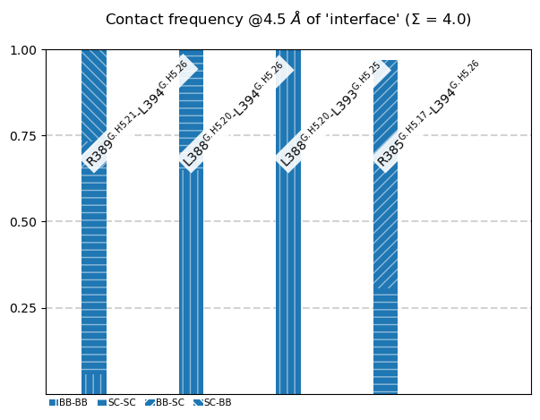
These are the contacts associated with the C-terminus of $:nbsphinx-math:`alpha`$5 bending back and interacting with itself:
   freq            label              residues  fragments   sum
1  1.00  R389@G.H5.21 - L394@G.H5.26  348 - 353    0 - 0   1.00
2  1.00  L388@G.H5.20 - L394@G.H5.26  347 - 353    0 - 0   2.00
3  1.00  L388@G.H5.20 - L393@G.H5.25  347 - 352    0 - 0   3.00
4  0.97  R385@G.H5.17 - L394@G.H5.26  344 - 353    0 - 0   3.97
We have also ploted them also as bars, including the atom-types.
Interfaces: AA_selection
If the fragments themselves are still too broad a definition, one can select a sub-set of aminoacids of those fragments via AA_selection:
From the docs
AA_selection : str or list, default is None
    Whatever the fragment definition and fragment selection
    has been, one can further refine the list of
    potential residue pairs by making a selection at
    the level of single aminoacids (AAs).
    E.g., if (like above) one has selected the interface
    to be "TM3" vs "TM2",

    >>> interface_selection_1="TM3"
    >>> interface_selection_2="TM2"

    but wants to select only some regions of those helices,
    one can pass here an `AA_selection`.
Please read the rest of the docs, since the parameter has more options than the ones we’re about to use.
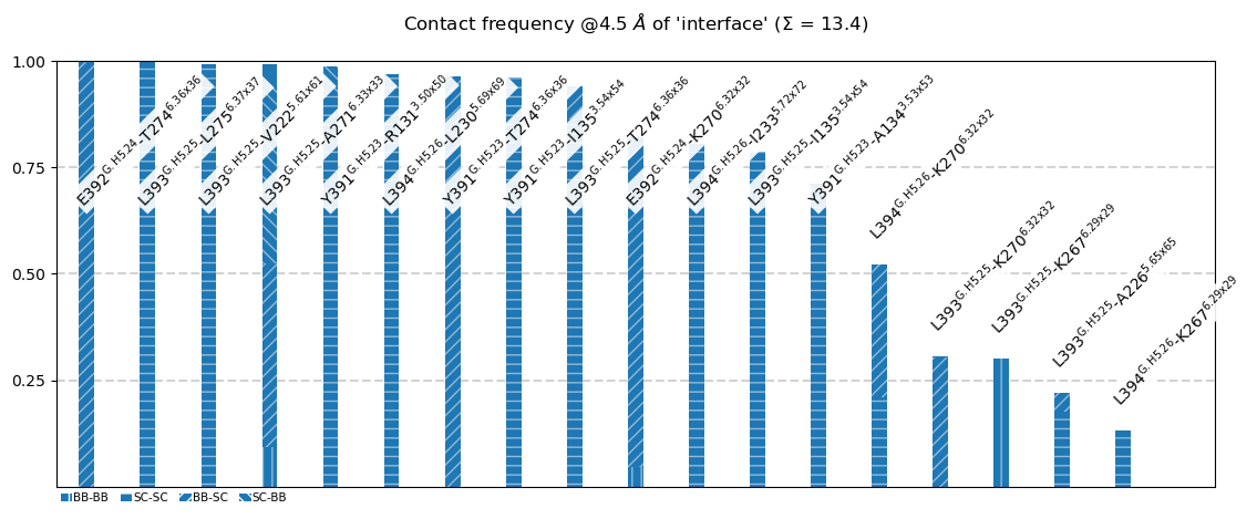
Here, we define the interface as contacts of the $:nbsphinx-math:`alpha`$5-helix of the G-protein with the TM-bundle, using
no_disk=True, interface_selection_1="G.H5", interface_selection_2="TM*"
and then use
AA_selection="390-394"
G.H5 with 26 AAs THR369@G.H5.01 ( 328) - LEU394@G.H5.26 (353 ) (G.H5)[12]:
intf = mdciao.cli.interface("mdciao_example/traj.xtc", topology="mdciao_example/top.pdb",
                            fragments="consensus",accept_guess=True,
                            no_disk=True, interface_selection_1="G.H5", interface_selection_2="TM*",
                            ctc_control=1.0,
                            GPCR_UniProt="adrb2_human",CGN_UniProt="gnas2_human",
                            n_nearest=4,
                            AA_selection="390-394",
                            figures=False)
intf.plot_freqs_as_bars(4.5, shorten_AAs=True, plot_atomtypes=True);
Will compute contact frequencies for trajectories:
mdciao_example/traj.xtc
 with a stride of 1 frames
Using method 'resSeq+' these fragments were found
fragment 0 with    354 AAs     LEU4 (   0) -   LEU394 (353 ) (0) resSeq jumps
fragment 1 with    340 AAs     GLN1 ( 354) -   ASN340 (693 ) (1)
fragment 2 with     66 AAs     ALA2 ( 694) -    PHE67 (759 ) (2)
fragment 3 with    284 AAs    GLU30 ( 760) -   P0G395 (1043) (3) resSeq jumps
No local file ./adrb2_human.xlsx found, checking online in
https://gpcrdb.org/services/residues/extended/adrb2_human ...done!
Please cite the following reference to the GPCRdb:
 * Kooistra et al, (2021) GPCRdb in 2021: Integrating GPCR sequence, structure and function
   Nucleic Acids Research 49, D335--D343
   https://doi.org/10.1093/nar/gkaa1080
For more information, call mdciao.nomenclature.references()
The GPCR-labels align best with fragments: [3] (first-last: GLU30-P0G395).

Mapping the GPCR fragments onto your topology:
 TM1  with     32 AAs    GLU30@1.29x29   ( 760) -    PHE61@1.60x60   (791 ) (TM1)
 ICL1 with      4 AAs    GLU62@12.48x48  ( 792) -    GLN65@12.51x51  (795 ) (ICL1)
 TM2  with     32 AAs    THR66@2.37x37   ( 796) -    LYS97@2.68x67   (827 ) (TM2)
 ECL1 with      4 AAs    MET98@23.49x49  ( 828) -   PHE101@23.52x52  (831 ) (ECL1)
 TM3  with     36 AAs   GLY102@3.21x21   ( 832) -   SER137@3.56x56   (867 ) (TM3)
 ICL2 with      8 AAs   PRO138@34.50x50  ( 868) -   LEU145@34.57x57  (875 ) (ICL2)
 TM4  with     27 AAs   THR146@4.38x38   ( 876) -   HIS172@4.64x64   (902 ) (TM4)
 ECL2 with     20 AAs   TRP173           ( 903) -   THR195           (922 ) (ECL2) resSeq jumps
 TM5  with     42 AAs   ASN196@5.35x36   ( 923) -   GLU237@5.76x76   (964 ) (TM5)
 ICL3 with      2 AAs   GLY238           ( 965) -   ARG239           (966 ) (ICL3)
 TM6  with     35 AAs   CYS265@6.27x27   ( 967) -   GLN299@6.61x61   (1001) (TM6)
 ECL3 with      4 AAs   ASP300           (1002) -   ILE303           (1005) (ECL3)
 TM7  with     25 AAs   ARG304@7.31x30   (1006) -   ARG328@7.55x55   (1030) (TM7)
 H8   with     12 AAs   SER329@8.47x47   (1031) -   LEU340@8.58x58   (1042) (H8)
No local file ./gnas2_human.xlsx found, checking online in
https://gpcrdb.org/services/residues/extended/gnas2_human ...done!
Please cite the following reference to the GPCRdb:
 * Kooistra et al, (2021) GPCRdb in 2021: Integrating GPCR sequence, structure and function
   Nucleic Acids Research 49, D335--D343
   https://doi.org/10.1093/nar/gkaa1080
Please cite the following reference to the CGN nomenclature:
 * Flock et al, (2015) Universal allosteric mechanism for G$\alpha$ activation by GPCRs
   Nature 2015 524:7564 524, 173--179
   https://doi.org/10.1038/nature14663
For more information, call mdciao.nomenclature.references()
The CGN-labels align best with fragments: [0] (first-last: LEU4-LEU394).

Mapping the CGN fragments onto your topology:
 G.HN   with     33 AAs     LEU4@G.HN.10   (   0) -    VAL36@G.HN.53   (32  ) (G.HN)
 G.hns1 with      3 AAs    TYR37@G.hns1.01 (  33) -    ALA39@G.hns1.03 (35  ) (G.hns1)
 G.S1   with      7 AAs    THR40@G.S1.01   (  36) -    LEU46@G.S1.07   (42  ) (G.S1)
 G.s1h1 with      6 AAs    GLY47@G.s1h1.01 (  43) -    GLY52@G.s1h1.06 (48  ) (G.s1h1)
 G.H1   with      7 AAs    LYS53@G.H1.01   (  49) -    GLN59@G.H1.07   (55  ) (G.H1)
 H.HA   with     26 AAs    LYS88@H.HA.04   (  56) -   LEU113@H.HA.29   (81  ) (H.HA)
 H.hahb with      9 AAs   VAL114@H.hahb.01 (  82) -   PRO122@H.hahb.09 (90  ) (H.hahb)
 H.HB   with     14 AAs   GLU123@H.HB.01   (  91) -   ASN136@H.HB.14   (104 ) (H.HB)
 H.hbhc with      7 AAs   VAL137@H.hbhc.01 ( 105) -   PRO143@H.hbhc.15 (111 ) (H.hbhc)
 H.HC   with     12 AAs   PRO144@H.HC.01   ( 112) -   GLU155@H.HC.12   (123 ) (H.HC)
 H.hchd with      1 AAs   ASP156@H.hchd.01 ( 124) -   ASP156@H.hchd.01 (124 ) (H.hchd)
 H.HD   with     12 AAs   GLU157@H.HD.01   ( 125) -   GLU168@H.HD.12   (136 ) (H.HD)
 H.hdhe with      5 AAs   TYR169@H.hdhe.01 ( 137) -   ASP173@H.hdhe.05 (141 ) (H.hdhe)
 H.HE   with     13 AAs   CYS174@H.HE.01   ( 142) -   LYS186@H.HE.13   (154 ) (H.HE)
 H.hehf with      7 AAs   GLN187@H.hehf.01 ( 155) -   SER193@H.hehf.07 (161 ) (H.hehf)
 H.HF   with      6 AAs   ASP194@H.HF.01   ( 162) -   ARG199@H.HF.06   (167 ) (H.HF)
 G.hfs2 with      5 AAs   CYS200@G.hfs2.01 ( 168) -   GLY206@G.hfs2.07 (172 ) (G.hfs2) resSeq jumps
 G.S2   with      8 AAs   ILE207@G.S2.01   ( 173) -   VAL214@G.S2.08   (180 ) (G.S2)
 G.s2s3 with      2 AAs   ASP215@G.s2s3.01 ( 181) -   LYS216@G.s2s3.02 (182 ) (G.s2s3)
 G.S3   with      8 AAs   VAL217@G.S3.01   ( 183) -   VAL224@G.S3.08   (190 ) (G.S3)
 G.s3h2 with      3 AAs   GLY225@G.s3h2.01 ( 191) -   GLN227@G.s3h2.03 (193 ) (G.s3h2)
 G.H2   with     10 AAs   ARG228@G.H2.01   ( 194) -   CYS237@G.H2.10   (203 ) (G.H2)
 G.h2s4 with      5 AAs   PHE238@G.h2s4.01 ( 204) -   THR242@G.h2s4.05 (208 ) (G.h2s4)
 G.S4   with      7 AAs   ALA243@G.S4.01   ( 209) -   ALA249@G.S4.07   (215 ) (G.S4)
 G.s4h3 with      8 AAs   SER250@G.s4h3.01 ( 216) -   ASN264@G.s4h3.15 (223 ) (G.s4h3) resSeq jumps
 G.H3   with     18 AAs   ARG265@G.H3.01   ( 224) -   LEU282@G.H3.18   (241 ) (G.H3)
 G.h3s5 with      3 AAs   ARG283@G.h3s5.01 ( 242) -   ILE285@G.h3s5.03 (244 ) (G.h3s5)
 G.S5   with      7 AAs   SER286@G.S5.01   ( 245) -   ASN292@G.S5.07   (251 ) (G.S5)
 G.s5hg with      1 AAs   LYS293@G.s5hg.01 ( 252) -   LYS293@G.s5hg.01 (252 ) (G.s5hg)
 G.HG   with     17 AAs   GLN294@G.HG.01   ( 253) -   ASP310@G.HG.17   (269 ) (G.HG)
 G.hgh4 with     21 AAs   TYR311@G.hgh4.01 ( 270) -   ASP331@G.hgh4.21 (290 ) (G.hgh4)
 G.H4   with     16 AAs   PRO332@G.H4.01   ( 291) -   ARG347@G.H4.17   (306 ) (G.H4)
 G.h4s6 with     11 AAs   ILE348@G.h4s6.01 ( 307) -   TYR358@G.h4s6.20 (317 ) (G.h4s6)
 G.S6   with      5 AAs   CYS359@G.S6.01   ( 318) -   PHE363@G.S6.05   (322 ) (G.S6)
 G.s6h5 with      5 AAs   THR364@G.s6h5.01 ( 323) -   ASP368@G.s6h5.05 (327 ) (G.s6h5)
 G.H5   with     26 AAs   THR369@G.H5.01   ( 328) -   LEU394@G.H5.26   (353 ) (G.H5)
Select group 1: G.H5
Select group 2: TM1, TM2, TM3, TM4, TM5, TM6, TM7

Will look for contacts in the interface between fragments
G.H5
and
TM1, TM2, TM3, TM4, TM5, TM6, TM7.

Excluding residue pairs not involving residues '390-394' (5 AAs) reduces from 5954 to 1145 residue pairs.

Performing a first pass on the 1145 group_1-group_2 residue pairs to compute lower bounds on residue-residue distances via residue-COM distances.
Reduced to only 165 (from 1145) residue pairs for the computation of actual residue-residue distances:
The following 18 contacts capture 13.40 (~98%) of the total frequency 13.64 (over 25 contacts with nonzero frequency at 4.50 Angstrom).
As orientation value, the first 14 ctcs already capture 90.0% of 13.64.
The 14-th contact has a frequency of 0.52.

    freq            label              residues  fragments   sum
1   1.00  E392@G.H5.24 - T274@6.36x36  351 - 976    0 - 3    1.00
2   1.00  L393@G.H5.25 - L275@6.37x37  352 - 977    0 - 3    2.00
3   0.99  L393@G.H5.25 - V222@5.61x61  352 - 949    0 - 3    2.99
4   0.99  L393@G.H5.25 - A271@6.33x33  352 - 973    0 - 3    3.98
5   0.99  Y391@G.H5.23 - R131@3.50x50  350 - 861    0 - 3    4.97
6   0.97  L394@G.H5.26 - L230@5.69x69  353 - 957    0 - 3    5.94
7   0.96  Y391@G.H5.23 - T274@6.36x36  350 - 976    0 - 3    6.90
8   0.96  Y391@G.H5.23 - I135@3.54x54  350 - 865    0 - 3    7.86
9   0.94  L393@G.H5.25 - T274@6.36x36  352 - 976    0 - 3    8.80
10  0.82  E392@G.H5.24 - K270@6.32x32  351 - 972    0 - 3    9.62
11  0.80  L394@G.H5.26 - I233@5.72x72  353 - 960    0 - 3   10.42
12  0.79  L393@G.H5.25 - I135@3.54x54  352 - 865    0 - 3   11.21
13  0.71  Y391@G.H5.23 - A134@3.53x53  350 - 864    0 - 3   11.92
14  0.52  L394@G.H5.26 - K270@6.32x32  353 - 972    0 - 3   12.44
15  0.31  L393@G.H5.25 - K270@6.32x32  352 - 972    0 - 3   12.75
16  0.30  L393@G.H5.25 - K267@6.29x29  352 - 969    0 - 3   13.05
17  0.22  L393@G.H5.25 - A226@5.65x65  352 - 953    0 - 3   13.27
18  0.13  L394@G.H5.26 - K267@6.29x29  353 - 969    0 - 3   13.40

          label  freq
1  L393@G.H5.25  5.54
2  Y391@G.H5.23  3.62
3  L394@G.H5.26  2.42
4  E392@G.H5.24  1.82

           label  freq
1   T274@6.36x36  2.90
2   I135@3.54x54  1.75
3   K270@6.32x32  1.65
4   L275@6.37x37  1.00
5   V222@5.61x61  0.99
6   A271@6.33x33  0.99
7   R131@3.50x50  0.99
8   L230@5.69x69  0.97
9   I233@5.72x72  0.80
10  A134@3.53x53  0.71
11  K267@6.29x29  0.43
12  A226@5.65x65  0.22
Finally
Some of these parameters/criteria appear in other places in mdciao, not only at the moment of computing the distances, but also at the moment of showing them. E.g., the method mdciao.flare.freqs2flare automatically hides neighboring contacts via the exclude_neighbors = 1 parameter.
So, if at any moment you miss some contact in the reports (graphical or otherwise), check if some of the parameters above are at play.