Comparing Contact Frequencies: Bar Plots
In this notebook, we present a walk-through of the methods for comparing frequencies. In particular, we will use mdciao.plots.compare_groups_of_contacts. And we will try to refine, step-by-step, the same comparison plot, focusing on what the individual parameters can do to show or hide information.
Note
In principle, mdciao tries to make sane decisions about hiding/showing information, but those do not cover all usecases and you’re encouraged to learn how to customize the plots to your liking.
The Data
We start off by loading previously computed domain interfaces for publicly available MD data of the Covid-19 Spike Protein, curated in the impressive COVID-19 Molecular Structure and Therapeutics Hub put together by the Molecular Sciences Software Institute (molSSI).
In particular, we use the data generated in the Chodera-Lab by Ivy Zhang, consisting of Folding@home simulations of the SARS-CoV-2 spike RBD bound to human ACE2 (725.3 µs ). We quote:
All-atom MD simulations of the SARS-CoV-2 spike protein receptor binding domain (RBD) bound to human angiotensin converting enzyme-related carboypeptidase (ACE2), simulated using Folding@Home. The “wild-type” RBD and three mutants (N439K, K417V, and the double mutant N439K/K417V) were simulated.…RUNs denote different RBD mutants: N439K (RUN0), K417V (RUN1), N439K/K417V (RUN2), and WT (RUN3). CLONEs denote different independent replica trajectories
We can get the pre-computed interfaces with mdciao:
[1]:
import mdciao
import mdtraj as md
import numpy as np
import os
if not os.path.exists("example_cov19"):
    mdciao.examples.fetch_example_data("cov19")
interfaces = np.load("example_cov19/interfaces.f_50.t_2.npy",allow_pickle=True)[()]
interfaces = {key:interfaces[key] for key in ['WT', 'K417V', 'N439K','N439K/K417V']}
Unzipping to 'example_cov19'
Please note that, to keep filesizes small and download times short, we use a very compressed version of the huge dataset: one in 50 frames, one in two trajectories.
Step-by-Step Refining of the Comparison-Plot
We will be comparing contact frequencies by repeatedly calling mdciao.plots.compare_groups_of_contacts, with the same input data, only tweaking some of the parameters each time. This will generate a lot of plots, which we display here for learning purposes, but, in principle, you could be iterating over the same notebook cell until you like what you see.
Note
Since the data is mutagenesis data, we need to pass along a mutations_dict so that mdciao knows that some residues are equivalent to each other even if they have different names:
mutations_dict={"V417": "K417",
                "K439": "N439"
               }
That, in itself, isn’t a parameter for refining the plot, but rather to ensure that the comparison can take place.
[2]:
mdciao.plots.compare_groups_of_contacts(interfaces,
                                        ctc_cutoff_Ang=3.5,
                                        mutations_dict={"V417": "K417",
                                                        "K439": "N439"
                                                       });
These interactions are not shared:
0LB752-K417, 0LB752-R408, 0LB752-Y505, 0YB754-D420, 0YB754-D427, 0YB754-K424, 0YB754-N460, 0YB754-R408, 0fA755-K417, 4YB751-E406, 4YB751-G416, 4YB751-K417, 4YB751-T415, A2750-G413, A2750-G416, A2750-Q409, A2750-Q414, A2750-R408, A2750-T415, A2753-D420, A2753-G413, A2753-G416, A2753-K417, A2753-N460, A2753-Q409, A2753-Q414, A2753-R408, A2753-Y421, A386-Y505, D30-K417, E37-R403, F490-K31, H34-K417, H34-R403, H34-S494, K31-L492, L79-Y489, Q24-S477
Their cumulative ctc freq is 21.02.
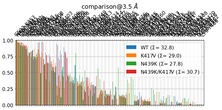
Wow! We can’t see anything. Let’s start refining the plot.
Figure Size
First, we simply make the figure a bit larger. There’s two ways of doing this:
Using figsize
[3]:
mdciao.plots.compare_groups_of_contacts(interfaces,
                                        ctc_cutoff_Ang=3.5,
                                        figsize=(25,5),
                                        mutations_dict={"V417": "K417",
                                                       "K439": "N439"
                                                       });
These interactions are not shared:
0LB752-K417, 0LB752-R408, 0LB752-Y505, 0YB754-D420, 0YB754-D427, 0YB754-K424, 0YB754-N460, 0YB754-R408, 0fA755-K417, 4YB751-E406, 4YB751-G416, 4YB751-K417, 4YB751-T415, A2750-G413, A2750-G416, A2750-Q409, A2750-Q414, A2750-R408, A2750-T415, A2753-D420, A2753-G413, A2753-G416, A2753-K417, A2753-N460, A2753-Q409, A2753-Q414, A2753-R408, A2753-Y421, A386-Y505, D30-K417, E37-R403, F490-K31, H34-K417, H34-R403, H34-S494, K31-L492, L79-Y489, Q24-S477
Their cumulative ctc freq is 21.02.
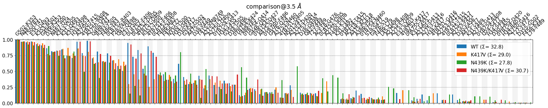
Much better already!
Using figsize is a good option when having a specific figure (or ratio) is important. For instance, when stacking several figures on top of each other, or filling in a specific a spot on the paper/slide/poster. However, there’s also the next option.
Using inch_per_contacts=1 (or some other numeric value) together with figsize=None
This fixes the amount of axis space each contact gets. When stacking plots on top of each other, some plots will be shorter and some will be longer, but the bars in them will have the same width and occupy the same amount of axis space and look equally wide.
[4]:
mdciao.plots.compare_groups_of_contacts(interfaces,
                                        ctc_cutoff_Ang=3.5,
                                        figsize=None,
                                        inch_per_contacts=1,
                                        mutations_dict={"V417": "K417",
                                                       "K439": "N439"
                                                       });
These interactions are not shared:
0LB752-K417, 0LB752-R408, 0LB752-Y505, 0YB754-D420, 0YB754-D427, 0YB754-K424, 0YB754-N460, 0YB754-R408, 0fA755-K417, 4YB751-E406, 4YB751-G416, 4YB751-K417, 4YB751-T415, A2750-G413, A2750-G416, A2750-Q409, A2750-Q414, A2750-R408, A2750-T415, A2753-D420, A2753-G413, A2753-G416, A2753-K417, A2753-N460, A2753-Q409, A2753-Q414, A2753-R408, A2753-Y421, A386-Y505, D30-K417, E37-R403, F490-K31, H34-K417, H34-R403, H34-S494, K31-L492, L79-Y489, Q24-S477
Their cumulative ctc freq is 21.02.

For now, we continue with with figsize and keep refining the plot.
[5]:
fig, freqs, plotted_freqs = mdciao.plots.compare_groups_of_contacts(interfaces,
                                                                    ctc_cutoff_Ang=3.5,
                                                                    figsize=(25,5) ,
                                                                    mutations_dict={"V417": "K417",
                                                                                    "K439": "N439"
                                                                                   });
These interactions are not shared:
0LB752-K417, 0LB752-R408, 0LB752-Y505, 0YB754-D420, 0YB754-D427, 0YB754-K424, 0YB754-N460, 0YB754-R408, 0fA755-K417, 4YB751-E406, 4YB751-G416, 4YB751-K417, 4YB751-T415, A2750-G413, A2750-G416, A2750-Q409, A2750-Q414, A2750-R408, A2750-T415, A2753-D420, A2753-G413, A2753-G416, A2753-K417, A2753-N460, A2753-Q409, A2753-Q414, A2753-R408, A2753-Y421, A386-Y505, D30-K417, E37-R403, F490-K31, H34-K417, H34-R403, H34-S494, K31-L492, L79-Y489, Q24-S477
Their cumulative ctc freq is 21.02.

Before continuing, some observations:
- The \(\Sigma\) values in the legend are simply the sum over all bar-heights for each system.These four values provide a way to estimate the average number of contacts involved in the RBD-ACE interface in each system. Their absolute value shouldn’t be taken too literally, since they’re
ctc_cutoff_Ang-dependent, but the differences among them can be informative. In this case, they point towards theWTsystem having around four more contacts on average than .eg. theK417Vsystem: \(\Sigma\) 32 vs. 28, respectively. Apart from plotting the figure, mdciao.plots.compare_groups_of_contacts also returns a tuple of three Python objects:
fig, freqs, plotted_freqs. From the documentation:myfig : :obj:`~matplotlib.pyplot.Figure` Figure with the comparison plot freqs : dictionary Unified frequency dictionaries, including mutations and anchor plotted_freqs : dictionary Like :obj:`freqs` but sorted and purged according to the user-defined input options, s.t. it represents the plotted valuesThis is very useful if we want to continue using the plotted values in the notebook, e.g. showing a formatted table using
pandasDataFrames:
[6]:
from pandas import DataFrame
DataFrame(plotted_freqs).round(3)
[6]:
| WT | K417V | N439K | N439K/K417V | mean | |
|---|---|---|---|---|---|
| G502-K353 | 0.998 | 0.999 | 0.995 | 0.997 | 1.00 |
| N487-Y83 | 0.963 | 0.966 | 0.968 | 0.969 | 0.97 |
| T500-Y41 | 0.953 | 0.971 | 0.920 | 0.962 | 0.95 |
| E35-Q493 | 0.972 | 0.964 | 0.909 | 0.961 | 0.95 |
| K353-N501 | 0.925 | 0.939 | 0.897 | 0.920 | 0.92 |
| ... | ... | ... | ... | ... | ... |
| A2750-G416 | 0.000 | 0.022 | 0.000 | 0.000 | 0.01 |
| T27-Y473 | 0.003 | 0.002 | 0.015 | 0.001 | 0.01 |
| D355-G502 | 0.003 | 0.006 | 0.003 | 0.002 | 0.00 |
| F456-K31 | 0.003 | 0.002 | 0.002 | 0.003 | 0.00 |
| L79-Y489 | 0.000 | 0.000 | 0.009 | 0.000 | 0.00 |
102 rows × 5 columns
Removing Identities
Next, we look at other ways of trimming the plot. We can, for instance, remove those contacts that are always formed in all systems. This effectively trims the plot from the left, hiding the contacts where where all four bars have heights larger or equal to a given value. This is loosely equivalent to a baseline removal. This is achieved with:
remove_identities=True,
identity_cutoff=1.
If we check the documentation:
remove_identities : bool, default is False
    If True, the contacts where
    freq[sys][ctc] >= :obj:`identity_cutoff`
    across all systems will not be plotted
    nor considered in the sum over contacts
identity_cutoff : float, default is 1
    If :obj:`remove_identities`, use this value to define what
    is considered an identity, s.t. contacts with values e.g. .95
    can also be removed
[7]:
mdciao.plots.compare_groups_of_contacts(interfaces,
                                        ctc_cutoff_Ang=3.5,
                                        figsize=(25,5),
                                        remove_identities=True,
                                        identity_cutoff=.80,
                                        mutations_dict={"V417": "K417",
                                                        "K439": "N439"
                                                       });
These interactions are not shared:
0LB752-K417, 0LB752-R408, 0LB752-Y505, 0YB754-D420, 0YB754-D427, 0YB754-K424, 0YB754-N460, 0YB754-R408, 0fA755-K417, 4YB751-E406, 4YB751-G416, 4YB751-K417, 4YB751-T415, A2750-G413, A2750-G416, A2750-Q409, A2750-Q414, A2750-R408, A2750-T415, A2753-D420, A2753-G413, A2753-G416, A2753-K417, A2753-N460, A2753-Q409, A2753-Q414, A2753-R408, A2753-Y421, A386-Y505, D30-K417, E37-R403, F490-K31, H34-K417, H34-R403, H34-S494, K31-L492, L79-Y489, Q24-S477
Their cumulative ctc freq is 21.02.
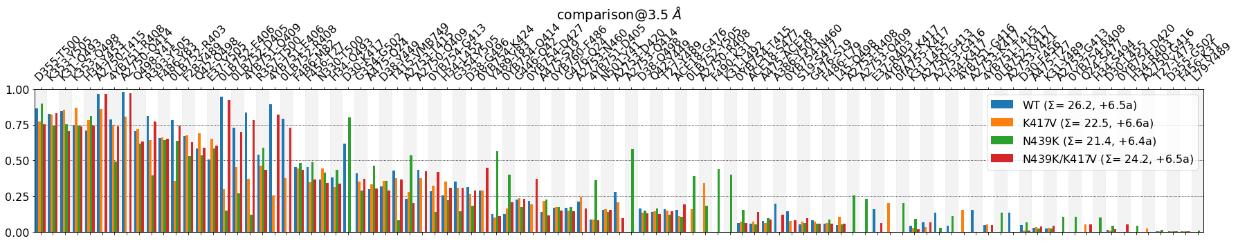
Some observations:
Choosing an
identity_cutoff=.80means we consider contacts that formed in over 80% (of the data of each setup) as formed as those contacts formed 100%. In our case, that means that the first six contacts have been hidden, up toG496-K353:
[8]:
DataFrame(plotted_freqs).round(3)[:7]
[8]:
| WT | K417V | N439K | N439K/K417V | mean | |
|---|---|---|---|---|---|
| G502-K353 | 0.998 | 0.999 | 0.995 | 0.997 | 1.00 |
| N487-Y83 | 0.963 | 0.966 | 0.968 | 0.969 | 0.97 |
| T500-Y41 | 0.953 | 0.971 | 0.920 | 0.962 | 0.95 |
| E35-Q493 | 0.972 | 0.964 | 0.909 | 0.961 | 0.95 |
| K353-N501 | 0.925 | 0.939 | 0.897 | 0.920 | 0.92 |
| G496-K353 | 0.907 | 0.942 | 0.870 | 0.918 | 0.91 |
| D355-T500 | 0.863 | 0.772 | 0.896 | 0.752 | 0.82 |
Note
In the above table we show the seventh row, D355-T500, to show that, even though the mean value of is over .80, the identity_cutoff>=.8 must apply to all systems, which is not the case. Hence, in the plot above the table, D355-T500 is the first shown contact
Continuing with the observations:
The \(\Sigma\) value is broken down into two contributions, e.g. for
WTit’s \(\Sigma\) = 26.2 + 5.7a. Those 5.7 are the approximately six hidden contacts that are above the identity cutoff.All four systems, i.e all four \(\Sigma\) values have hidden the same six contacts, s.t. the difference of approximately four contacts between
WTandK417Vis conserved: 26 vs 22, respectively.
Removing Small Values
We continue trimming the plot, now hiding negligible contributions using the argument lower_cutoff_val. This is somehow trimming from the right (of the panel), i.e. removing the long tail of small bars from the plot:
[9]:
mdciao.plots.compare_groups_of_contacts(interfaces,
                                        ctc_cutoff_Ang=3.5,
                                        figsize=(25,5),
                                        remove_identities=True,
                                        identity_cutoff=.80,
                                        mutations_dict={"V417": "K417",
                                                        "K439": "N439"
                                                       },
                                       lower_cutoff_val=.25
                                       );
These interactions are not shared:
0LB752-K417, 0LB752-R408, 0LB752-Y505, 0YB754-D420, 0YB754-D427, 0YB754-K424, 0YB754-N460, 0YB754-R408, 0fA755-K417, 4YB751-E406, 4YB751-G416, 4YB751-K417, 4YB751-T415, A2750-G413, A2750-G416, A2750-Q409, A2750-Q414, A2750-R408, A2750-T415, A2753-D420, A2753-G413, A2753-G416, A2753-K417, A2753-N460, A2753-Q409, A2753-Q414, A2753-R408, A2753-Y421, A386-Y505, D30-K417, E37-R403, F490-K31, H34-K417, H34-R403, H34-S494, K31-L492, L79-Y489, Q24-S477
Their cumulative ctc freq is 21.02.
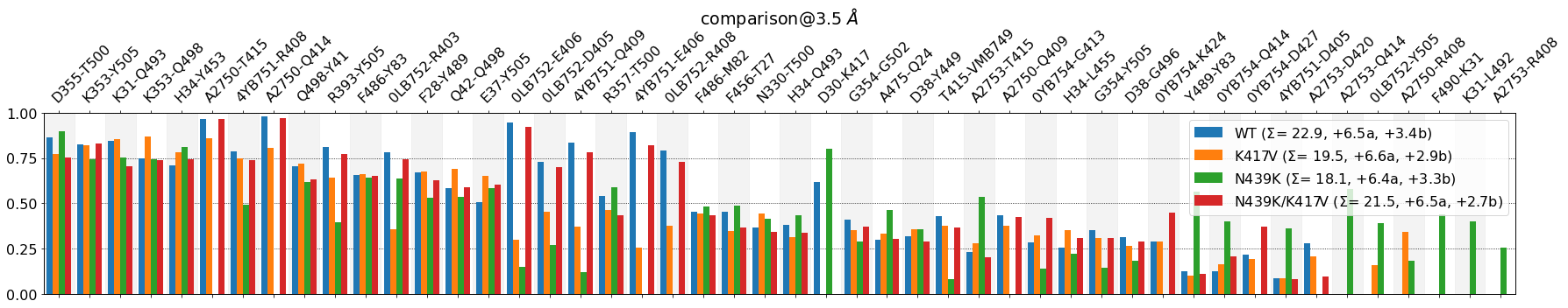
Some observations:
The plot is shorter from the right, there’s no contacts where all bars are below .25
\(\Sigma\) values are again broken into one more term, e.g. for
WT: \(\Sigma\) = 23.6 +5.7a +2.6b. Those 2.6 are the sum of the hidden bars, which are below (= b ) the cutoffThe difference of approximately 4 contacts on average between
WTandK417Vis still somewhat conserved between 23.6 and 20.2, respectively
If we really don’t want the legend to be that large (it can get distracting), we can turn it off with verbose_legend=False:
[10]:
mdciao.plots.compare_groups_of_contacts(interfaces,
                                        ctc_cutoff_Ang=3.5,
                                        figsize=(25,5),
                                        remove_identities=True,
                                        identity_cutoff=.80,
                                        mutations_dict={"V417": "K417",
                                                        "K439": "N439"
                                                       },
                                        lower_cutoff_val=.25,
                                        verbose_legend=False,
                                       );
These interactions are not shared:
0LB752-K417, 0LB752-R408, 0LB752-Y505, 0YB754-D420, 0YB754-D427, 0YB754-K424, 0YB754-N460, 0YB754-R408, 0fA755-K417, 4YB751-E406, 4YB751-G416, 4YB751-K417, 4YB751-T415, A2750-G413, A2750-G416, A2750-Q409, A2750-Q414, A2750-R408, A2750-T415, A2753-D420, A2753-G413, A2753-G416, A2753-K417, A2753-N460, A2753-Q409, A2753-Q414, A2753-R408, A2753-Y421, A386-Y505, D30-K417, E37-R403, F490-K31, H34-K417, H34-R403, H34-S494, K31-L492, L79-Y489, Q24-S477
Their cumulative ctc freq is 21.02.
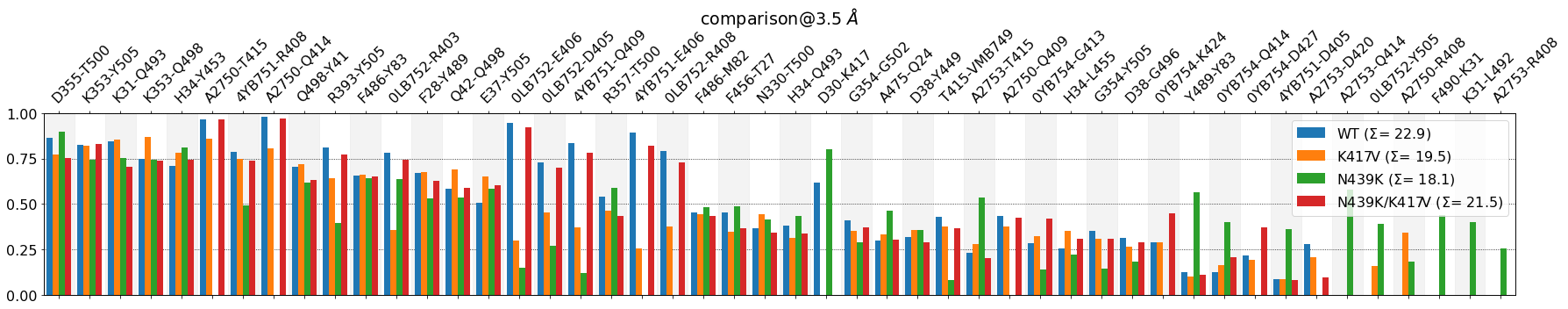
Visual Aides
Still, the plot contains a lot of information. We can make some of it stand out using a color code on the contact labels. The keyword is assign_w_color=True and the color-code is as follows:
- Only one system is present, i.e. its frequency is above the
lower_cutoff_value:Color the label with the system’s color and prepend it with “+” - Only one system is absent, i.e. its frequency is below the
lower_cutoff_value:Color the label with the system’s color and prepend it with “-”
[11]:
mdciao.plots.compare_groups_of_contacts(interfaces,
                                        ctc_cutoff_Ang=3.5,
                                        figsize=(25,5),
                                        remove_identities=True,
                                        identity_cutoff=.80,
                                        mutations_dict={"V417": "K417",
                                                        "K439": "N439"
                                                       },
                                        lower_cutoff_val=.25,
                                        verbose_legend=False,
                                        assign_w_color=True,
                                       );
These interactions are not shared:
0LB752-K417, 0LB752-R408, 0LB752-Y505, 0YB754-D420, 0YB754-D427, 0YB754-K424, 0YB754-N460, 0YB754-R408, 0fA755-K417, 4YB751-E406, 4YB751-G416, 4YB751-K417, 4YB751-T415, A2750-G413, A2750-G416, A2750-Q409, A2750-Q414, A2750-R408, A2750-T415, A2753-D420, A2753-G413, A2753-G416, A2753-K417, A2753-N460, A2753-Q409, A2753-Q414, A2753-R408, A2753-Y421, A386-Y505, D30-K417, E37-R403, F490-K31, H34-K417, H34-R403, H34-S494, K31-L492, L79-Y489, Q24-S477
Their cumulative ctc freq is 21.02.
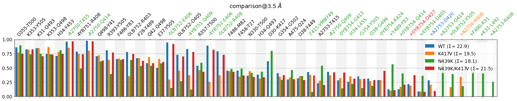
Some observations:
N439Kis missing a some contacts that are more present in the other systems, likeA2750-T415, A2570-Q414, 4YB51-E406but has gained some other contacts only present inN439:Y489-Y83, F490-K31, K31-L492This loss of contacts is captured in part by
N439K’s \(\Sigma\) being the lowest of all.The color code is not a definitive guide to what’s important on the plot, but rather a short-hand for quick visual inspection. It misses some things like contacts where two systems are missing, and it’s coupled to the
lower_cutoff_valparameter.Even without the color code, it’s somewhat easy to locate contacts the behavior is very different across systems, e.g. the salt bridge
D30-K147and so on.
There’s more ways of highlighting these types of highly variant contacts, we will touch on that later, but let’s continue consolidating the plot.
Consolidating the Plot
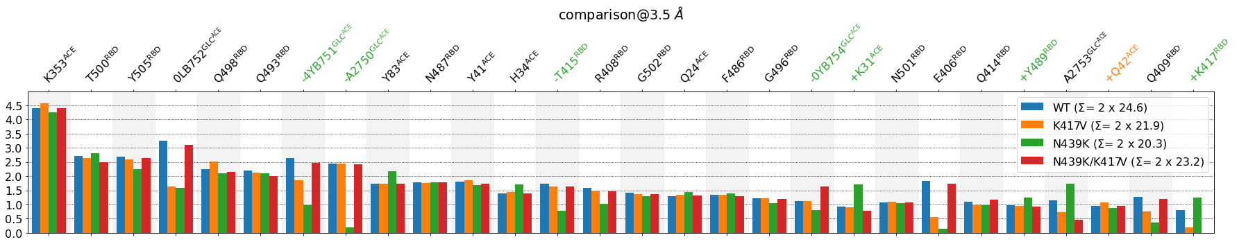
We can further summarize the interface comparison at the cost of losing some information. We can aggregate contact frequencies by residue, so that we no longer look at individual residue-pairs, but rather at each residue’s participation in the interface. We do that with per_residue=True.
[12]:
mdciao.plots.compare_groups_of_contacts(interfaces,
                                        ctc_cutoff_Ang=3.5,
                                        figsize=(25,5),
                                        remove_identities=True,
                                        identity_cutoff=.80,
                                        mutations_dict={"V417": "K417",
                                                        "K439": "N439"
                                                       },
                                        lower_cutoff_val=.25,
                                        verbose_legend=False,
                                        assign_w_color=True,
                                        per_residue=True,
                                       );
These interactions are not shared:
0fA755, A386, D420, D427, F490, G416, K417, K424, L492, N460, S494, Y421
Their cumulative ctc freq is 7.55.
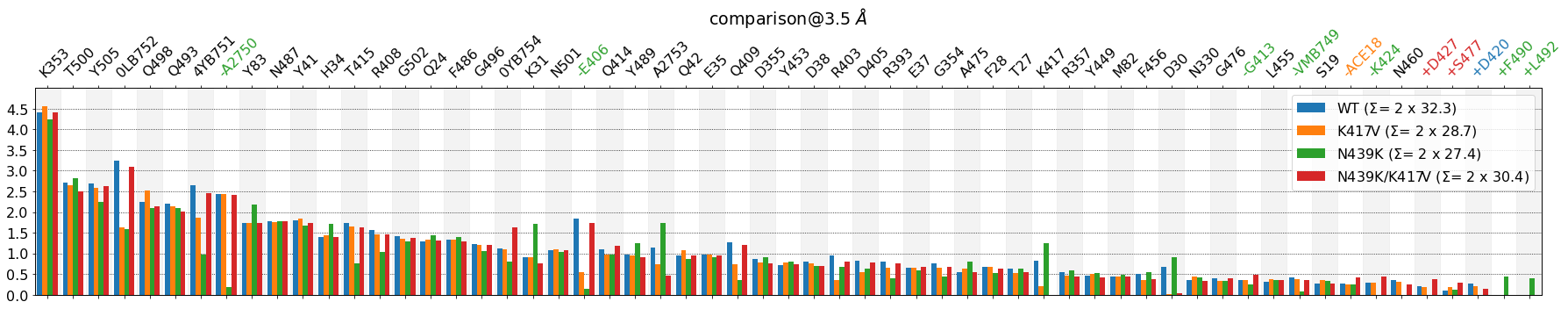
Some observations:
K353stands out as the most involved residue in the interface, across all setupsA2750andE406don’t participate in the interface inN439Kmutant\(\Sigma\) values are represented as 2 x 31.4 (e.g. for
WT), because the actual sum of the represented bars is 62.8, but the number of involved contacts is half of that.remove_identitiesis left without effect (it’s in the documentation of the method)lower_cutoff_valworks as expected
Showing Fragment Information: Informative Labels
So far, we’ve been hiding the fragment information, i.e., to what molecular fragments [ACE, RBD and/or their glycans GLC@ACE and GLC@RBD] a given residue belongs to. That’s because mdciao.plots.compare_groups_of_contacts uses defrag=@ by default. This parameter tells mdciao that, in the contact labels, residues have been affiliated to their fragments
using the @-symbol and that we want to use that information to remove (defrag) those affiliations from the labels, typically to make labels more compact. Using defrag=None yields:
[13]:
mdciao.plots.compare_groups_of_contacts(interfaces,
                                        ctc_cutoff_Ang=3.5,
                                        figsize=(25,5),
                                        remove_identities=True,
                                        identity_cutoff=.80,
                                        mutations_dict={"V417": "K417",
                                                        "K439": "N439"
                                                       },
                                        lower_cutoff_val=1,
                                        verbose_legend=False,
                                        assign_w_color=True,
                                        per_residue=True,
                                        defrag=None,
                                       );
These interactions are not shared:
0fA755@GLC^ACE, A386@ACE, D420@RBD, D427@RBD, F490@RBD, G416@RBD, K417@RBD, K424@RBD, L492@RBD, N460@RBD, S494@RBD, Y421@RBD
Their cumulative ctc freq is 7.55.
Some observations:
Now the labels include the fragment, e.g.
E406@RBDorA2750@GLC_ACE.lower_cutoff_val=1hides those residues involved, on average, in less than one interface-contact.
Using Fragment Information: Sorting by Interface Side
Still, we can continue tweaking the plot to separate residues according to what side of the interface they are on. Setting interface=True tells mdciao that the mdciao.contacts.ContactGroup-objects contained the in variable interfaces can be assigned to one of the two sides of an interface.
This is possible because in the original notebook these ContactGroups were initialized using mdciao.cli.interface.
[14]:
mdciao.plots.compare_groups_of_contacts(interfaces,
                                        ctc_cutoff_Ang=3.5,
                                        figsize=(25,5),
                                        remove_identities=True,
                                        identity_cutoff=.80,
                                        mutations_dict={"V417": "K417",
                                                        "K439": "N439"
                                                       },
                                        lower_cutoff_val=1,
                                        verbose_legend=False,
                                        assign_w_color=True,
                                        per_residue=True,
                                        defrag=None,
                                        interface=True
                                       );
These interactions are not shared:
0fA755@GLC^ACE, A386@ACE, D420@RBD, D427@RBD, F490@RBD, G416@RBD, K417@RBD, K424@RBD, L492@RBD, N460@RBD, S494@RBD, Y421@RBD
Their cumulative ctc freq is 7.55.
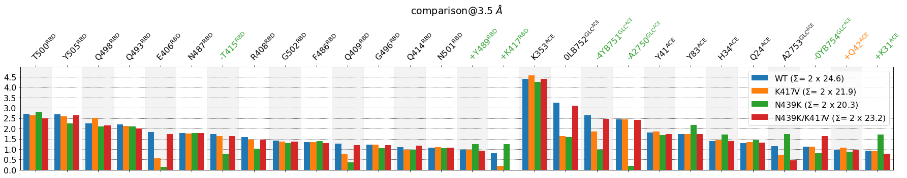
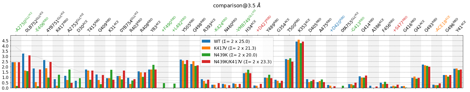
The sorting now puts first the residues belonging to the [RBD,GLC@RBD]-side followed by those belonging to [ACE,GLC@ACE]-side. This immediately informs about the residues that participate the most in the interface between domains, namely, for the RBD: T500, Y505 and for the ACE: K353 by far, then three glycans, one of them severely impacted by the N439K mutation.
Sorting by Standard Deviation
So far, contacts have been shown in descending order of mean frequency values, i.e., those contacts most formed are shown first, those less formed are shown last, which seems natural if the goal is to characterize the interface itself.
However, our goal is also easily spot diferences across setups, in this case the effect of the mutations K417V, N439K, N439K/K417.
We can do that with sort_by=std. First, let’s see how that affects all contacts (without cutoffs, identites or whatever), and then we will trim it down as we did above:
[15]:
mdciao.plots.compare_groups_of_contacts(interfaces,
                                        ctc_cutoff_Ang=3.5,
                                        figsize=(25,5),
                                        mutations_dict={"V417": "K417",
                                                        "K439": "N439"
                                                       },
                                        verbose_legend=False,
                                        assign_w_color=True,
                                        sort_by="std",
                                       );
These interactions are not shared:
0LB752-K417, 0LB752-R408, 0LB752-Y505, 0YB754-D420, 0YB754-D427, 0YB754-K424, 0YB754-N460, 0YB754-R408, 0fA755-K417, 4YB751-E406, 4YB751-G416, 4YB751-K417, 4YB751-T415, A2750-G413, A2750-G416, A2750-Q409, A2750-Q414, A2750-R408, A2750-T415, A2753-D420, A2753-G413, A2753-G416, A2753-K417, A2753-N460, A2753-Q409, A2753-Q414, A2753-R408, A2753-Y421, A386-Y505, D30-K417, E37-R403, F490-K31, H34-K417, H34-R403, H34-S494, K31-L492, L79-Y489, Q24-S477
Their cumulative ctc freq is 21.02.
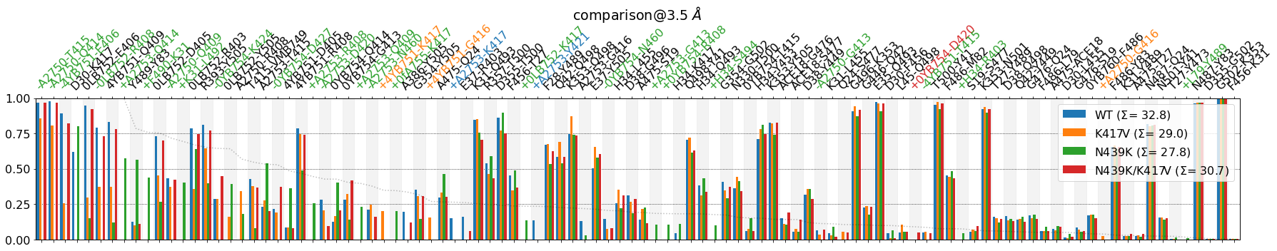
Some observations, since the plot looks quite different:
At the rightmost edge, we have the least variant contacts (low standard deviation, std), regardless of the contacts themselves being highly conserved (
G502-K353, 100% across systems) or barely there (Q42-Y449, 15% across systems)At the leftmost edge, we have the most variant contacts (high std), e.g.
A2750-T415is almost fully present in three systems, and fully absent in one.There’s a faint dotted line descending horizontally in the background. That line is the numerical value of the std itself. The reason for plotting it is that now
lower_cutoff_valoperates on the std itself, not on the mean frequency. From the docs:
sort_by : str, default is "mean"
    The property by which to sort the contacts.
    It is always descending and the property can be:
     * "mean" sort by mean frequency over all systems, making most
       frequent contacts appear on the left/top of the plot.
     * "std" sort by per-contact standard deviation over all systems, making
       the contacts with most different values appear on top. This
       highlights more "deviant" contacts and might hence be
       more informative than "mean" in cases where a lot of
       contacts have similar frequencies (high or low). If this option
       is activated, a faint dotted line is incorporated into the plot
       that marks the std for each contact group
[...]
lower_cutoff_val : float, default is 0
    Hide contacts with small values. "values" changes
    meaning depending on :obj:`sort_by`. If :obj:`sort_by` is:
     * "mean" or "keep" or "numeric", then hide contacts where **all**
       systems have frequencies lower than this value.
     * "std", then hide contacts where the standard
       deviation across systems *itself* is lower than this value.
       This hides contacts where all systems are
       similar, regardless of whether they're all
       around 1, around .5 or around 0
Meaning, by looking at the faint dotted line, we can decide what lower_cutoff_val we want to use to truncate the plot from the right, e.g. lower_cutoff_val=.25. We can also include now defrag=None since the plot will be less crowded and also legend_rows=2, to make the legend less invasive:
[16]:
mdciao.plots.compare_groups_of_contacts(interfaces,
                                        ctc_cutoff_Ang=3.5,
                                        figsize=(25,5),
                                        mutations_dict={"V417": "K417",
                                                        "K439": "N439"
                                                       },
                                        verbose_legend=False,
                                        assign_w_color=True,
                                        sort_by="std",
                                        lower_cutoff_val=.25,
                                        defrag=None,
                                        legend_rows=2
                                       );
These interactions are not shared:
0LB752@GLC^ACE-K417@RBD, 0LB752@GLC^ACE-R408@RBD, 0LB752@GLC^ACE-Y505@RBD, 0YB754@GLC^ACE-D420@RBD, 0YB754@GLC^ACE-D427@RBD, 0YB754@GLC^ACE-K424@RBD, 0YB754@GLC^ACE-N460@RBD, 0YB754@GLC^ACE-R408@RBD, 0fA755@GLC^ACE-K417@RBD, 4YB751@GLC^ACE-E406@RBD, 4YB751@GLC^ACE-G416@RBD, 4YB751@GLC^ACE-K417@RBD, 4YB751@GLC^ACE-T415@RBD, A2750@GLC^ACE-G413@RBD, A2750@GLC^ACE-G416@RBD, A2750@GLC^ACE-Q409@RBD, A2750@GLC^ACE-Q414@RBD, A2750@GLC^ACE-R408@RBD, A2750@GLC^ACE-T415@RBD, A2753@GLC^ACE-D420@RBD, A2753@GLC^ACE-G413@RBD, A2753@GLC^ACE-G416@RBD, A2753@GLC^ACE-K417@RBD, A2753@GLC^ACE-N460@RBD, A2753@GLC^ACE-Q409@RBD, A2753@GLC^ACE-Q414@RBD, A2753@GLC^ACE-R408@RBD, A2753@GLC^ACE-Y421@RBD, A386@ACE-Y505@RBD, D30@ACE-K417@RBD, E37@ACE-R403@RBD, F490@RBD-K31@ACE, H34@ACE-K417@RBD, H34@ACE-R403@RBD, H34@ACE-S494@RBD, K31@ACE-L492@RBD, L79@ACE-Y489@RBD, Q24@ACE-S477@RBD
Their cumulative ctc freq is 21.02.
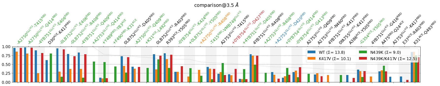
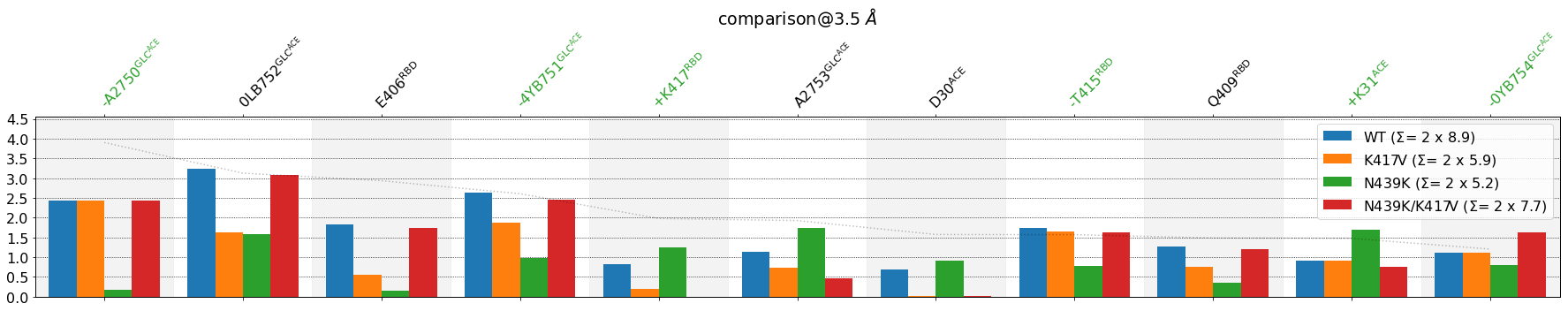
The leftmost part of the plot is filled with highly variant contacts, where the mutation N439K has most impacted the interface in the ACE-glycans.
If we now combine this with per_residue=True:
[17]:
mdciao.plots.compare_groups_of_contacts(interfaces,
                                        ctc_cutoff_Ang=3.5,
                                        figsize=(25,5),
                                        mutations_dict={"V417": "K417",
                                                        "K439": "N439"
                                                       },
                                        verbose_legend=False,
                                        assign_w_color=True,
                                        sort_by="std",
                                        lower_cutoff_val=.25,
                                        defrag=None,
                                        per_residue=True,
                                       );
These interactions are not shared:
0fA755@GLC^ACE, A386@ACE, D420@RBD, D427@RBD, F490@RBD, G416@RBD, K417@RBD, K424@RBD, L492@RBD, N460@RBD, S494@RBD, Y421@RBD
Their cumulative ctc freq is 7.55.
The lower_cutoff_val needs to be tweaked again, since aggregating frequencies by residue results in higher values being shown, which results in other, usually higher, std values. Again, we use the faint dotted line to help us choose the value: lower_cutoff_val=1:
[18]:
mdciao.plots.compare_groups_of_contacts(interfaces,
                                        ctc_cutoff_Ang=3.5,
                                        figsize=(25,5),
                                        mutations_dict={"V417": "K417",
                                                        "K439": "N439"
                                                       },
                                        verbose_legend=False,
                                        assign_w_color=True,
                                        sort_by="std",
                                        lower_cutoff_val=1,
                                        per_residue=True,
                                        defrag=None,
                                       );
These interactions are not shared:
0fA755@GLC^ACE, A386@ACE, D420@RBD, D427@RBD, F490@RBD, G416@RBD, K417@RBD, K424@RBD, L492@RBD, N460@RBD, S494@RBD, Y421@RBD
Their cumulative ctc freq is 7.55.
Coloring
Finally, if the colors have been bothering you, you can either pass them along directly or choose from matplotlib’s colormaps:
colors : iterable (list or dict), or str, default is None
    * If list, the colors will be assigned in the same
      order of :obj:`groups`.
    * If dict, has to have the
      same keys as :obj:`groups`.
    * If str, it has to be a case-sensitve colormap-name of matplotlib:
      https://matplotlib.org/stable/tutorials/colors/colormaps.html
    * If None, the 'tab10' colormap (tableau) is chosen
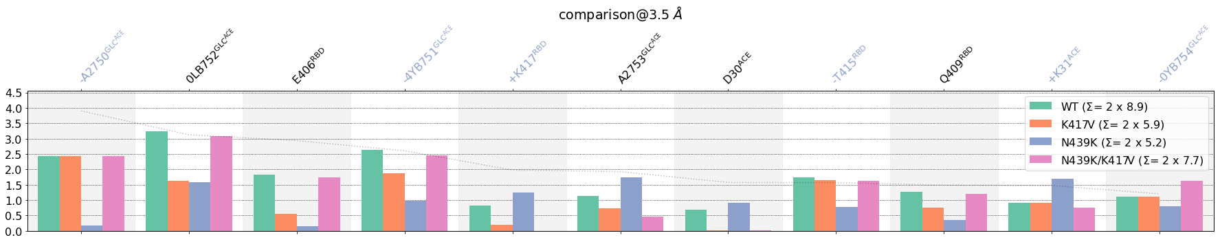
[19]:
mdciao.plots.compare_groups_of_contacts(interfaces,
                                        ctc_cutoff_Ang=3.5,
                                        figsize=(25,5),
                                        mutations_dict={"V417": "K417",
                                                        "K439": "N439"
                                                       },
                                        verbose_legend=False,
                                        assign_w_color=True,
                                        sort_by="std",
                                        lower_cutoff_val=1,
                                        per_residue=True,
                                        defrag=None,
                                        colors="Set2"
                                       );
These interactions are not shared:
0fA755@GLC^ACE, A386@ACE, D420@RBD, D427@RBD, F490@RBD, G416@RBD, K417@RBD, K424@RBD, L492@RBD, N460@RBD, S494@RBD, Y421@RBD
Their cumulative ctc freq is 7.55.