Missing Contacts
You might find that some contacts that you were expecting to be found by mdciao don’t actually show up in mdciao’s results. Several input parameters control the contact reporting of mdciao, and it might not be obvious which one of them (if any) is actually hiding your contact. The logic behind these parameters, and their default values, is fairly straightforward, and we illustrate it here.
If you want to run this notebook on your own, please download and extract the data from here first. You can download it:
using the browser
using the terminal with
wget http://proteinformatics.org/mdciao/mdciao_example.zip; unzip mdciao_example.zipusing mdciao’s own method mdciao.examples.fetch_example_data
If you want to take a 3D-look at this data, you can do it here.
ctc_cutoff_Ang
This is the most obvious parameter that controls the contact computation. It appears virtually in all methods (CLI or API) that compute contact frequencies. Whenever it has a default value, it is 3.5 Angstrom.
Note
Please see the note of caution on the use of hard cutoffs in the main page of the docs.
[1]:
import mdciao, os
if not os.path.exists("mdciao_example"):
    mdciao.examples.fetch_example_data()
[2]:
import mdtraj as md
traj = md.load("mdciao_example/traj.xtc",top="mdciao_example/prot.pdb")
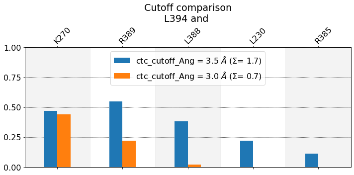
First, we individually call mdciao.cli.residue_neighborhoods with two ctc_cutoff_Ang values, 3.0 and 3.5 Angstrom. This will generate two frequency reports which we will later compare with mdciao.cli.compare. Please refer to those methods if their function calls aren’t entirely
clear to you.
[3]:
from io import StringIO
from contextlib import redirect_stdout
b = StringIO()
with redirect_stdout(b):
    for ctc_cutoff_Ang in [3, 3.5]:
        mdciao.cli.residue_neighborhoods("L394",traj,
                                         short_AA_names=True,
                                         ctc_cutoff_Ang=ctc_cutoff_Ang,
                                         figures=False,
                                         fragment_names=None,
                                         no_disk=False)
mdciao.cli.compare({
    "ctc_cutoff_Ang = 3.5 AA" : "neighborhood.LEU394@3.5_Ang.dat",
    "ctc_cutoff_Ang = 3.0 AA" : "neighborhood.LEU394@3.0_Ang.dat",
                   },
                   anchor="L394",
                  title="Cutoff comparison");
b.close()
These interactions are not shared:
L230, R385
Their cumulative ctc freq is 0.33.
Created files
freq_comparison.pdf
freq_comparison.xlsx
Note
We are hiding most outputs with the use of redirect_stdout.
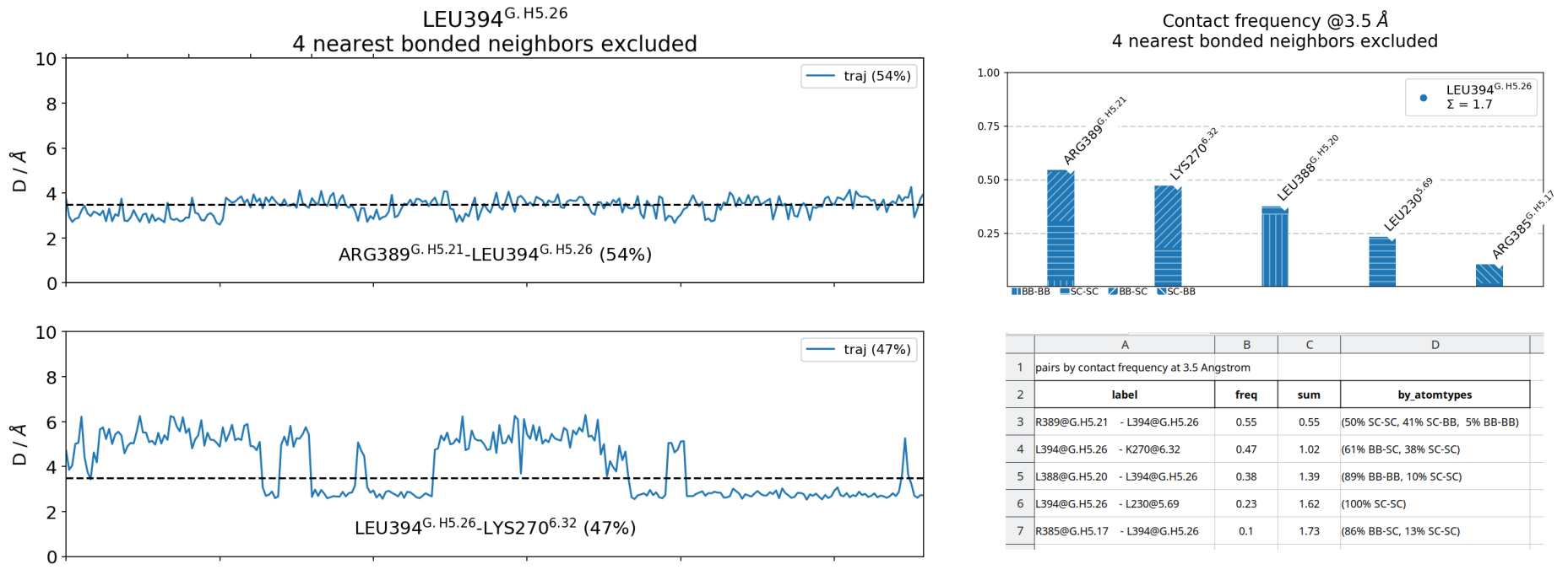
We observe that the smaller the cutoff, the fewer contacts get reported. In this case L230 and R385 never approach L394 at distances smaller than 3.0 Angstrom during in the entire simulation, hence they don’t get reported. As for K270, the frequency doesn’t change very much, because it’s a salt-bridge that’s really either formed at very close distance or broken at higher distances, as can be seen in this time-trace
figure. Also notice that, at 3.5 Angstrom, the sum over bars, \(\Sigma\), is higher, since the height of the bars has increased.
ctc_control
Even when using the same ctc_cutoff_Ang, there’s other ways of controlling what gets reported. ctc_control is one of them. This parameter controls how many residues get reported per neighborhood, since usually one is not interested in all residues but only the most frequent ones.
Controlling with integers
One way to control this is to select only the first n frequent ones (n is an integer and is 5 by default). Here we do the comparison again:
[4]:
b = StringIO()
ctc_cutoff_Ang = 3.5
ctc_controls = [3,4,5,6]
with redirect_stdout(b):
    for ctc_control in ctc_controls:
        mdciao.cli.residue_neighborhoods("L394",traj,
                                         short_AA_names=True,
                                         ctc_cutoff_Ang=ctc_cutoff_Ang,
                                         ctc_control=ctc_control,
                                         figures=False,
                                         fragment_names=None,
                                         no_disk=False,
                                         output_desc='neighborhood.ctc_control_%u'%ctc_control)
mdciao.cli.compare({"ctc-control = %u"%key : "neighborhood.ctc_control_%u.LEU394@%2.1f_Ang.dat"%(key,ctc_cutoff_Ang)
                   for key in ctc_controls},
                   anchor="L394",
                  title="ctc-control comparison");
b.close()
These interactions are not shared:
I233, L230, R385
Their cumulative ctc freq is 0.92.
Created files
freq_comparison.pdf
freq_comparison.xlsx
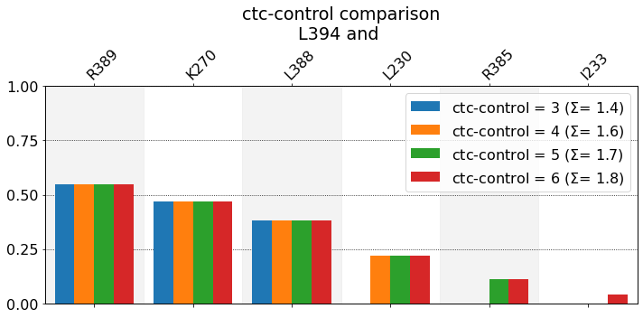
n is simply the number of reported bars: three blue ones, four orange ones, five green ones, and six red ones. \(\Sigma\) is just the sum of the heights of all bars and is thus an estimate of the average number of neighbors that are being reported (at this cutoff). A couple of observations:
The relation of \(\Sigma\) with n is straightforward: as n grows, so does \(\Sigma\).
For a fixed cutoff, there’s an upper bond to \(\Sigma\) (\(\Sigma\leq\Sigma_t\)), because the total average number of neighbors, \(\Sigma_t\), of a given residue, over a given dataset, is determined by the used cutoff only. The
ctc_controlparameter simply determines how many neighbors get actually reported.Because neighbors get reported by descending frequency, the neighbors that get left out when chosen n = 4 over n = of 5 or 6 are very likely not that significant. Please note that this won’t hold for very small datasets (like one single pdb file), where the word frequency doesn’t really have a defined meaning.
In cases where
mdciaois used to look for the neighborhood of just one residue, there’s a sensible number of residues to choose (somewhere between 5 and 10), because usually that’s how many interactions a residue will have (please note, this doesn’t necessary hold for elongated ligands, lipids, acid chains etc).
Actually, although it’s hidden above, mdciao reports to the terminal the percentage of \(\Sigma_t\) that the report captures, so that the user can decided whether to increase n or not, so for each of the iterations above, here are terminal-output excerpts:
ctc_control = 3
#idx   freq      contact       fragments     res_idxs      ctc_idx  Sum
1:     0.55   LEU394-ARG389       0-0         353-348        30     0.55
2:     0.47   LEU394-LYS270       0-3         353-972        65     1.02
3:     0.38   LEU394-LEU388       0-0         353-347        29     1.39
These 3 contacts capture 1.39 (~79%) of the total frequency 1.76 (over 74 input contacts)
As orientation value, the first 4 ctcs already capture 90.0% of 1.76.
The 4-th contact has a frequency of 0.23
The intention is to report how much of \(\Sigma_t\) has been captured using 3 contacts (~79%), and how many would be needed to capture most (90%) of it (4 contacts). So, as we increase n:
ctc_control = 4
#idx   freq      contact       fragments     res_idxs      ctc_idx  Sum
1:     0.55   LEU394-ARG389       0-0         353-348        30     0.55
2:     0.47   LEU394-LYS270       0-3         353-972        65     1.02
3:     0.38   LEU394-LEU388       0-0         353-347        29     1.39
4:     0.23   LEU394-LEU230       0-3         353-957        51     1.62
These 4 contacts capture 1.62 (~92%) of the total frequency 1.76 (over 74 input contacts)
ctc_control = 5
#idx   freq      contact       fragments     res_idxs      ctc_idx  Sum
1:     0.55   LEU394-ARG389       0-0         353-348        30     0.55
2:     0.47   LEU394-LYS270       0-3         353-972        65     1.02
3:     0.38   LEU394-LEU388       0-0         353-347        29     1.39
4:     0.23   LEU394-LEU230       0-3         353-957        51     1.62
5:     0.10   LEU394-ARG385       0-0         353-344        26     1.73
These 5 contacts capture 1.73 (~98%) of the total frequency 1.76 (over 74 input contacts)
ctc_control = 6
#idx   freq      contact       fragments     res_idxs      ctc_idx  Sum
1:     0.55   LEU394-ARG389       0-0         353-348        30     0.55
2:     0.47   LEU394-LYS270       0-3         353-972        65     1.02
3:     0.38   LEU394-LEU388       0-0         353-347        29     1.39
4:     0.23   LEU394-LEU230       0-3         353-957        51     1.62
5:     0.10   LEU394-ARG385       0-0         353-344        26     1.73
6:     0.04   LEU394-ILE233       0-3         353-960        54     1.76
These 6 contacts capture 1.76 (~100%) of the total frequency 1.76 (over 74 input contacts)
Controlling with fractions
Additionally, the upper bond itself, \(\Sigma_t\), can be used as a reference for controlling how many contacts get reported. So, instead of specifying an absolute number (n = 3,4,5…), one can specify a relative number, i.e. a fraction of \(\Sigma_t\) to be reported.
This way, regardless of the actual number of involved contacts, one can choose to report most of them. In the example below, we choose to report 90% of the total number of average neighbors, which, as we know from above, is achieved with 4 contacts. To avoid introducing a new parameter, mdciao knows that if ctc_control is an integer (1, 2, 3…), the user means this many contacts, whereas if ctc_control is between 0 and 1 (.50 for 50%, .9 for 90% etc) the user wants that fraction
of \(\Sigma_t\):
[5]:
mdciao.cli.residue_neighborhoods("L394",traj,
                                 short_AA_names=True,
                                 ctc_cutoff_Ang=ctc_cutoff_Ang,
                                 ctc_control=.90,
                                 figures=False,
                                 fragment_names=None,
                                 no_disk=False,
                                 );
Will compute contact frequencies for (1 items):
<mdtraj.Trajectory with 280 frames, 8384 atoms, 1044 residues, and unitcells>
 with a stride of 1 frames
Using method 'lig_resSeq+' these fragments were found
fragment      0 with    354 AAs     LEU4 (     0) -   LEU394 (353   ) (0)  resSeq jumps
fragment      1 with    340 AAs     GLN1 (   354) -   ASN340 (693   ) (1)
fragment      2 with     66 AAs     ALA2 (   694) -    PHE67 (759   ) (2)
fragment      3 with    283 AAs    GLU30 (   760) -   LEU340 (1042  ) (3)  resSeq jumps
fragment      4 with      1 AAs   P0G395 (  1043) -   P0G395 (1043  ) (4)

Will compute neighborhoods for the residues
L394
excluding 4 nearest neighbors

   residue      residx    fragment      resSeq       GPCR        CGN
    LEU394         353           0        394       None       None

Pre-computing likely neighborhoods by reducing the neighbor-list
to those within 15 Angstrom in the first frame of reference geom
'<mdtraj.Trajectory with 1 frames, 8384 atoms, 1044 residues, and unitcells>':...done!
From 1035 potential distances, the neighborhoods have been reduced to only 74 potential contacts.
If this number is still too high (i.e. the computation is too slow), consider using a smaller nlist_cutoff_Ang
Streaming over trajectory object nr.   0 (   280 frames,    280 with stride  1) in chunks of 10000 frames. Now at chunk nr    0, frames so far    280
#idx   freq      contact       fragments     res_idxs      ctc_idx  Sum
1:     0.55   LEU394-ARG389       0-0         353-348        30     0.55
2:     0.47   LEU394-LYS270       0-3         353-972        65     1.02
3:     0.38   LEU394-LEU388       0-0         353-347        29     1.40
4:     0.23   LEU394-LEU230       0-3         353-957        51     1.62
These 4 contacts capture 1.62 (~92%) of the total frequency 1.76 (over 74 input contacts)
./neighborhood.LEU394@3.5_Ang.dat
Which control-mode to choose (fraction or integers) is up to the user:
For compactness, limiting the output with integers can avoid huge outputs, but might leave out some interesting stuff.
For completeness, choosing
ctc_control = .99will ensure that any-residue under the cutoff (regardless of its frequency) will be reported, but might fill the reports with “long tails” of many residues with very low frequencies.
n_nearest
Another way in which mdciao is choosing which residues to show is through excluding nearest neighbors, i.e. residues that are predictably going to be under the cutoff simply because they are bonded neighbors of the residue in question.
In our example, for L394 these would be residues 395 and 393 (first bonded) 396 and 392 (second bonded) and so on (except, in this particular L394 case, since it’s a terminal residue, we only get 393, 392 etc). By the way, the meaning of bonded can be clarified
The default value that mdciao has this parameter is n_nearest=4 by default, which is approximately one \(\alpha\)-helix turn away. The intention is to avoid reporting up to the first helix away from the residue.
Let’s see the effect of varying this parameter:
[6]:
b = StringIO()
ctc_cutoff_Ang = 4.5
n_nearests = [0, 1, 2, 3, 4]
with redirect_stdout(b):
    for n_nearest in n_nearests:
        n = mdciao.cli.residue_neighborhoods("L394",traj,
                                         short_AA_names=True,
                                         ctc_cutoff_Ang=ctc_cutoff_Ang,
                                         ctc_control=20,
                                         n_nearest=n_nearest,
                                         figures=False,
                                         fragment_names=None,
                                         no_disk=False,
                                         output_desc='neighborhood.n_nearest_%u'%n_nearest)
mdciao.cli.compare({"n_n = %u"%key : "neighborhood.n_nearest_%u.LEU394@%2.1f_Ang.dat"%(key,ctc_cutoff_Ang)
                   for key in n_nearests},
                   anchor="L394",
                   title="n_neighbors comparison");
b.close()
These interactions are not shared:
E392, L393
Their cumulative ctc freq is 3.00.
Created files
freq_comparison.pdf
freq_comparison.xlsx
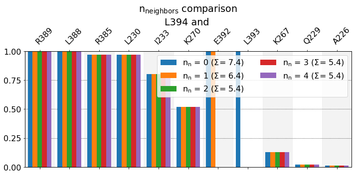
We can see also here that, the lower n_neighbors, i.e. the less neighbors we exclude, the higher the \(\Sigma\) value. With n_neighbors=0, in the report we see E392 and L393, both with full bars. Since L393 is covalently bonded to L394, thi sis expected (and hence not particularly informative). While L392 is not bonded to L394, there’s a strong expectation for it to be near L394, so this is also not very informative. So, as n_neighbors goes up, these
two bars get hidden, and the graph doesn’t change anymore. If you’re wondering what’s with position 391, there’s a TYR that points away from L394 throughout the simulation, so it wouldn’t appear on the report regardless.
nlist_cutoff_Ang
In order to speed up computations, mdciao creates an initial neighborlist from the topology file, or the first frame of the trajectory when no topology is passed. Only residues that are within nlist_cutoff_Ang in that frame are considered potential neighbors, s.t. non-necessary distances between distant domains aren’t unnecessarily computed, like the N-term of a receptor and Gamma sub-unit of a G-protein. This is admittedly risky in some cases, and will likely change in future versions
of mdciao (perhaps using kdtrees), but in general it works well if no large conformational changes take place during the simulation.
Conveniently, mdciao informs about this in the output by saying (e.g. in the terminal output from above):
Pre-computing likely neighborhoods by reducing the neighbor-list
to those within 15 Angstrom in the first frame of reference geom
'<mdtraj.Trajectory with 1 frames, 8384 atoms, 1044 residues, and unitcells>':...done!
From 1035 potential distances, the neighborhoods have been reduced to only 74 potential contacts.
If this number is still too high (i.e. the computation is too slow), consider using a smaller nlist_cutoff_Ang
Some known cases where the assumption that initial neighborhood (up to nlist_cutoff_Ang Angstrom) already contains all potential neighbors doesn’t hold:
binding simulations: If in your first frame the binding partners are far apart, but get closer during your simulation, the actual neighbors will be missing in the initial neighborlist. Binding partners can be anything: ligand and substrate, protein A and protein B, sub-unit \(\alpha\) and \(\beta\), whatever you want. In these cases, you can either use the final frame of the simulation as a reference frame, or simply increase the
nlist_cutoff_Angto a value that captures all possible contacts, although this might slow down the computation.docking data: Docking data might contain many different poses where the ligand is sampling not only the orthosteric binding pocket, but anything else found by the algorithm. Since there’s no single one representative frame for all this poses, you have to increase
nlist_cutoff_Angfor this.randomized-data: In general, any type of data where there’s a strong expectation of large conformational variability, beyond local rearrangements contained in the
nlist_cutoff_Ang, should be handled carefully.
interface_cutoff_Ang
When computing whole interfaces, rather than just residue neighborhoods, nlist_cutoff_Ang is called interface_cutoff_Ang, but it’s the same concept. Since the user is no longer looking at individual residue neighborhoods, but rather entire interfaces between molecular fragments, i.e. (sub) domains consisting of many residues, we assume that larger conformational changes are expected and thus set the default value at 35 Angstrom.
Finally
Some of these parameters/criteria appear in other places in mdciao, not only at the moment of computing the distances, but also at the moment of showing them. E.g., the method mdciao.cli.flare.freqs2flare automatically hides neighboring contacts via the exclude_neighbors = 1 parameter.
So, if at any moment you miss some contact in the reports (graphical or otherwise), check if some of the parameters above are at play.